Why use a Cluster?

Overview

Teaching: 15 min
Exercises: 5 min

Questions

• Why would I be interested in High Performance Computing (HPC)?

• What can I expect to learn from this course?

Objectives

• Be able to describe what an HPC system is

• Identify how an HPC system could benefit you.

Frequently, research problems that use computing can outgrow the capabilities of the desktop or laptop computer where they started:

• A statistics student wants to cross-validate a model. This involves running the model 1000 times — but each run takes an hour. Running the model on a laptop will take over a month! In this research problem, final results are calculated after all 1000 models have run, but typically only one model is run at a time (in serial) on the laptop. Since each of the 1000 runs is independent of all others, and given enough computers, it’s theoretically possible to run them all at once (in parallel).
• A genomics researcher has been using small datasets of sequence data, but soon will be receiving a new type of sequencing data that is 10 times as large. It’s already challenging to open the datasets on a computer — analyzing these larger datasets will probably crash it. In this research problem, the calculations required might be impossible to parallelize, but a computer with more memory would be required to analyze the much larger future data set.
• An engineer is using a fluid dynamics package that has an option to run in parallel. So far, this option was not used on a desktop. In going from 2D to 3D simulations, the simulation time has more than tripled. It might be useful to take advantage of that option or feature. In this research problem, the calculations in each region of the simulation are largely independent of calculations in other regions of the simulation. It’s possible to run each region’s calculations simultaneously (in parallel), communicate selected results to adjacent regions as needed, and repeat the calculations to converge on a final set of results. In moving from a 2D to a 3D model, both the amount of data and the amount of calculations increases greatly, and it’s theoretically possible to distribute the calculations across multiple computers communicating over a shared network.

In all these cases, access to more (and larger) computers is needed. Those computers should be usable at the same time, solving many researchers’ problems in parallel.

Break the Ice

Talk to your neighbour, office mate or rubber duck about your research.

• How does computing help you do your research?
• How could more computing help you do more or better research?

A Standard Laptop for Standard Tasks

Today, people coding or analysing data typically work with laptops.

Let’s dissect what resources programs running on a laptop require:

• the keyboard and/or touchpad is used to tell the computer what to do (Input)
• the internal computing resources Central Processing Unit and Memory perform calculation
• the display depicts progress and results (Output)

Schematically, this can be reduced to the following:

When Tasks Take Too Long

When the task to solve becomes heavy on computations, the operations are typically out-sourced from the local laptop or desktop to elsewhere. Take for example the task to find the directions for your next vacation. The capabilities of your laptop are typically not enough to calculate that route spontaneously: finding the shortest path through a network runs on the order of (v log v) time, where v (vertices) represents the number of intersections in your map. Instead of doing this yourself, you use a website, which in turn runs on a server, that is almost definitely not in the same room as you are.

Note here, that a server is mostly a noisy computer mounted into a rack cabinet which in turn resides in a data center. The internet made it possible that these data centers do not require to be nearby your laptop. What people call the cloud is mostly a web-service where you can rent such servers by providing your credit card details and requesting remote resources that satisfy your requirements. This is often handled through an online, browser-based interface listing the various machines available and their capacities in terms of processing power, memory, and storage.

The server itself has no direct display or input methods attached to it. But most importantly, it has much more storage, memory and compute capacity than your laptop will ever have. In any case, you need a local device (laptop, workstation, mobile phone or tablet) to interact with this remote machine, which people typically call ‘a server’.

When One Server Is Not Enough

If the computational task or analysis to complete is daunting for a single server, larger agglomerations of servers are used. These go by the name of “clusters” or “super computers”.

The methodology of providing the input data, configuring the program options, and retrieving the results is quite different to using a plain laptop. Moreover, using a graphical interface is often discarded in favor of using the command line. This imposes a double paradigm shift for prospective users asked to

1. work with the command line interface (CLI), rather than a graphical user interface (GUI)
2. work with a distributed set of computers (called nodes) rather than the machine attached to their keyboard & mouse

I’ve Never Used a Server, Have I?

Take a minute and think about which of your daily interactions with a computer may require a remote server or even cluster to provide you with results.

Some Ideas

• Checking email: your computer (possibly in your pocket) contacts a remote machine, authenticates, and downloads a list of new messages; it also uploads changes to message status, such as whether you read, marked as junk, or deleted the message. Since yours is not the only account, the mail server is probably one of many in a data center.
• Searching for a phrase online involves comparing your search term against a massive database of all known sites, looking for matches. This “query” operation can be straightforward, but building that database is a monumental task! Servers are involved at every step.
• Searching for directions on a mapping website involves connecting your (A) starting and (B) end points by traversing a graph in search of the “shortest” path by distance, time, expense, or another metric. Converting a map into the right form is relatively simple, but calculating all the possible routes between A and B is expensive.

Checking email could be serial: your machine connects to one server and exchanges data. Searching by querying the database for your search term (or endpoints) could also be serial, in that one machine receives your query and returns the result. However, assembling and storing the full database is far beyond the capability of any one machine. Therefore, these functions are served in parallel by a large, “hyperscale” collection of servers working together.

Key Points

• High Performance Computing (HPC) typically involves connecting to very large computing systems elsewhere in the world.

• These other systems can be used to do work that would either be impossible or much slower on smaller systems.

• The standard method of interacting with such systems is via a command line interface.

Working on a remote HPC system

Overview

Teaching: 25 min
Exercises: 10 min

Questions

• What is an HPC system?

• How does an HPC system work?

• How do I log in to a remote HPC system?

Objectives

• Connect to a remote HPC system.

• Understand the general HPC system architecture.

What Is an HPC System?

The words “cloud”, “cluster”, and the phrase “high-performance computing” or “HPC” are used a lot in different contexts and with various related meanings. So what do they mean? And more importantly, how do we use them in our work?

The cloud is a generic term commonly used to refer to computing resources that are a) provisioned to users on demand or as needed and b) represent real or virtual resources that may be located anywhere on Earth. For example, a large company with computing resources in Brazil, Zimbabwe and Japan may manage those resources as its own internal cloud and that same company may also use commercial cloud resources provided by Amazon or Google. Cloud resources may refer to machines performing relatively simple tasks such as serving websites, providing shared storage, providing web services (such as e-mail or social media platforms), as well as more traditional compute intensive tasks such as running a simulation.

The term HPC system, on the other hand, describes a stand-alone resource for computationally intensive workloads. They are typically comprised of a multitude of integrated processing and storage elements, designed to handle high volumes of data and/or large numbers of floating-point operations (FLOPS) with the highest possible performance. For example, all of the machines on the Top-500 list are HPC systems. To support these constraints, an HPC resource must exist in a specific, fixed location: networking cables can only stretch so far, and electrical and optical signals can travel only so fast.

The word “cluster” is often used for small to moderate scale HPC resources less impressive than the Top-500. Clusters are often maintained in computing centers that support several such systems, all sharing common networking and storage to support common compute intensive tasks.

Logging In

The first step in using a cluster is to establish a connection from our laptop to the cluster. When we are sitting at a computer (or standing, or holding it in our hands or on our wrists), we have come to expect a visual display with icons, widgets, and perhaps some windows or applications: a graphical user interface, or GUI. Since computer clusters are remote resources that we connect to over often slow or laggy interfaces (WiFi and VPNs especially), it is more practical to use a command-line interface, or CLI, in which commands and results are transmitted via text, only. Anything other than text (images, for example) must be written to disk and opened with a separate program.

If you have ever opened the Windows Command Prompt or macOS Terminal, you have seen a CLI. If you have already taken The Carpentries’ courses on the UNIX Shell or Version Control, you have used the CLI on your local machine somewhat extensively. The only leap to be made here is to open a CLI on a remote machine, while taking some precautions so that other folks on the network can’t see (or change) the commands you’re running or the results the remote machine sends back. We will use the Secure SHell protocol (or SSH) to open an encrypted network connection between two machines, allowing you to send & receive text and data without having to worry about prying eyes.

Make sure you have a SSH client installed on your laptop. Refer to the setup section for more details. SSH clients are usually command-line tools, where you provide the remote machine address as the only required argument. If your username on the remote system differs from what you use locally, you must provide that as well. If your SSH client has a graphical front-end, such as PuTTY or MobaXterm, you will set these arguments before clicking “connect.” From the terminal, you’ll write something like ssh userName@hostname, where the “@” symbol is used to separate the two parts of a single argument.

Go ahead and open your terminal or graphical SSH client, then log in to the cluster using your username and the remote computer you can reach from the outside world, NTNU,Trondheim, Norway.

[user@laptop ~]$ ssh MY_USER_NAME@saga.sigma2.no

Remember to replace MY_USER_NAME with your username or the one supplied by the instructors. You may be asked for your password. Watch out: the characters you type after the password prompt are not displayed on the screen. Normal output will resume once you press Enter.

Where Are We?

Very often, many users are tempted to think of a high-performance computing installation as one giant, magical machine. Sometimes, people will assume that the computer they’ve logged onto is the entire computing cluster. So what’s really happening? What computer have we logged on to? The name of the current computer we are logged onto can be checked with the hostname command. (You may also notice that the current hostname is also part of our prompt!)

[yourUsername@login-1.SAGA ~]$ hostname

login-1.SAGA

What’s in Your Home Directory?

The system administrators may have configured your home directory with some helpful files, folders, and links (shortcuts) to space reserved for you on other filesystems. Take a look around and see what you can find.

Hint: The shell commands pwd and ls may come in handy.

Home directory contents vary from user to user. Please discuss any differences you spot with your neighbors:

It’s a Beautiful Day in the Neighborhood

The deepest layer should differ: MY_USER_NAME is uniquely yours. Are there differences in the path at higher levels?

If both of you have empty directories, they will look identical. If you or your neighbor has used the system before, there may be differences. What are you working on?

Solution

Use pwd to print the working directory path:

[yourUsername@login-1.SAGA ~]$ pwd

You can run ls to list the directory contents, though it’s possible nothing will show up (if no files have been provided). To be sure, use the -a flag to show hidden files, too.

[yourUsername@login-1.SAGA ~]$ ls -a

At a minimum, this will show the current directory as ., and the parent directory as ...

Nodes

Individual computers that compose a cluster are typically called nodes (although you will also hear people call them servers, computers and machines). On a cluster, there are different types of nodes for different types of tasks. The node where you are right now is called the head node, login node, landing pad, or submit node. A login node serves as an access point to the cluster.

As a gateway, it is well suited for uploading and downloading files, setting up software, and running quick tests. Generally speaking, the login node should not be used for time-consuming or resource-intensive tasks. You should be alert to this, and check with your site’s operators or documentation for details of what is and isn’t allowed. In these lessons, we will avoid running jobs on the head node.

The real work on a cluster gets done by the worker (or compute) nodes. Worker nodes come in many shapes and sizes, but generally are dedicated to long or hard tasks that require a lot of computational resources.

All interaction with the worker nodes is handled by a specialized piece of software called a scheduler (the scheduler used in this lesson is called ). We’ll learn more about how to use the scheduler to submit jobs next, but for now, it can also tell us more information about the worker nodes.

For example, we can view all of the worker nodes by running the command sinfo.

[yourUsername@login-1.SAGA ~]$ sinfo

PARTITION AVAIL  TIMELIMIT  NODES  STATE NODELIST
normal*      up 7-00:00:00      1  down* c5-12
normal*      up 7-00:00:00     87    mix c1-[7,13-15,19,22-24,28,31,33,3.......
normal*      up 7-00:00:00    110  alloc c1-[1-6,8-9,11-12,16-18,20-21,........
normal*      up 7-00:00:00      1   idle c1-10
bigmem       up 14-00:00:0      1  drain c6-3
bigmem       up 14-00:00:0     10    mix c3-[29-31,53,56],c6-[1,4-7]
bigmem       up 14-00:00:0      1  alloc c6-2
bigmem       up 14-00:00:0     24   idle c3-[32-52,54-55],c6-8
accel        up 14-00:00:0      3    mix c7-[1-2,8]
accel        up 14-00:00:0      5  alloc c7-[3-7]
optimist     up   infinite      1  down* c5-12
optimist     up   infinite      1  drain c6-3
optimist     up   infinite    100    mix c1-[7,13-15,19,22-24,28,31,33,35,37...
optimist     up   infinite    116  alloc c1-[1-6,8-9,11-12,16-18,20-21,25-27...
optimist     up   infinite     25   idle c1-10,c3-[32-52,54-55],c6-8

There are also specialized machines used for managing disk storage, user authentication, and other infrastructure-related tasks. Although we do not typically logon to or interact with these machines directly, they enable a number of key features like ensuring our user account and files are available throughout the HPC system.

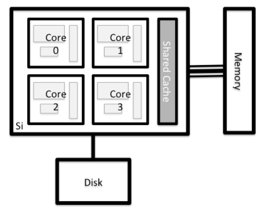
What’s in a Node?

All of the nodes in an HPC system have the same components as your own laptop or desktop: CPUs (sometimes also called processors or cores), memory (or RAM), and disk space. CPUs are a computer’s tool for actually running programs and calculations. Information about a current task is stored in the computer’s memory. Disk refers to all storage that can be accessed like a file system. This is generally storage that can hold data permanently, i.e. data is still there even if the computer has been restarted. While this storage can be local (a hard drive installed inside of it), it is more common for nodes to connect to a shared, remote fileserver or cluster of servers.

Explore Your Computer

Try to find out the number of CPUs and amount of memory available on your personal computer.

Note that, if you’re logged in to the remote computer cluster, you need to log out first. To do so, type Ctrl+d or exit:

[yourUsername@login-1.SAGA ~]$ exit
[user@laptop ~]$

Solution

There are several ways to do this. Most operating systems have a graphical system monitor, like the Windows Task Manager. More detailed information can be found on the command line:

• Run system utilities

  [user@laptop ~]$ nproc --all
  [user@laptop ~]$ free -m
  

• Read from /proc

  [user@laptop ~]$ cat /proc/cpuinfo
  [user@laptop ~]$ cat /proc/meminfo
  

• Run system monitor

  [user@laptop ~]$ htop
  

Explore the Head Node

Now compare the resources of your computer with those of the head node.

Solution

[user@laptop ~]$ ssh MY_USER_NAME@saga.sigma2.no
[yourUsername@login-1.SAGA ~]$ nproc --all
[yourUsername@login-1.SAGA ~]$ free -m

You can get more information about the processors using lscpu, and a lot of detail about the memory by reading the file /proc/meminfo:

[yourUsername@login-1.SAGA ~]$ less /proc/meminfo

You can also explore the available filesystems using df to show disk free space. The -h flag renders the sizes in a human-friendly format, i.e., GB instead of B. The type flag -T shows what kind of filesystem each resource is.

[yourUsername@login-1.SAGA ~]$ df -Th

The local filesystems (ext, tmp, xfs, zfs) will depend on whether you’re on the same login node (or compute node, later on). Networked filesystems (beegfs, cifs, gpfs, nfs, pvfs) will be similar — but may include MY_USER_NAME, depending on how it is mounted.

Shared Filesystems

This is an important point to remember: files saved on one node (computer) are often available everywhere on the cluster!

Explore a Worker Node

Finally, let’s look at the resources available on the worker nodes where your jobs will actually run. Try running this command to see the name, CPUs and memory available on the worker nodes (the instructors will give you the ID of the compute node to use):

 sinfo --node c3-12 -o "%n %c %m"

Compare Your Computer, the Head Node and the Worker Node

Compare your laptop’s number of processors and memory with the numbers you see on the cluster head node and worker node. Discuss the differences with your neighbor.

What implications do you think the differences might have on running your research work on the different systems and nodes?

Differences Between Nodes

Many HPC clusters have a variety of nodes optimized for particular workloads. Some nodes may have larger amount of memory, or specialized resources such as Graphical Processing Units (GPUs).

With all of this in mind, we will now cover how to talk to the cluster’s scheduler, and use it to start running our scripts and programs!

Key Points

• An HPC system is a set of networked machines.

• HPC systems typically provide login nodes and a set of worker nodes.

• The resources found on independent (worker) nodes can vary in volume and type (amount of RAM, processor architecture, availability of network mounted filesystems, etc.).

• Files saved on one node are available on all nodes.

Working with the scheduler

Overview

Teaching: 45 min
Exercises: 30 min

Questions

• What is a scheduler and why are they used?

• How do I launch a program to run on any one node in the cluster?

• How do I capture the output of a program that is run on a node in the cluster?

Objectives

• Run a simple Hello World style program on the cluster.

• Submit a simple Hello World style script to the cluster.

• Use the batch system command line tools to monitor the execution of your job.

• Inspect the output and error files of your jobs.

Job Scheduler

An HPC system might have thousands of nodes and thousands of users. How do we decide who gets what and when? How do we ensure that a task is run with the resources it needs? This job is handled by a special piece of software called the scheduler. On an HPC system, the scheduler manages which jobs run where and when.

The following illustration compares these tasks of a job scheduler to a waiter in a restaurant. If you can relate to an instance where you had to wait for a while in a queue to get in to a popular restaurant, then you may now understand why sometimes your job do not start instantly as in your laptop.

Job Scheduling Roleplay (Optional)

Your instructor will divide you into groups taking on different roles in the cluster (users, compute nodes and the scheduler). Follow their instructions as they lead you through this exercise. You will be emulating how a job scheduling system works on the cluster.

Instructions

To do this exercise, you will need about 50-100 pieces of paper or sticky notes.

1. Divide the room into groups, with specific roles.
   • Pick three or four people to be the “scheduler.”
   • Select one-third of the room be “users”, given several slips of paper (or post-it notes) and pens.
   • Have the remaining two thirds of the room be “compute nodes.”
   • Have the “users” go to the front of the room (or the back, wherever there’s space for them to stand) and the “schedulers” stand between the users and “compute nodes” (who should remain at their seats).

2. Divide the pieces of paper / sticky notes among the “users” and have them fill out all the pages with simple math problems and their name. Tell everyone that these are the jobs that need to be done and correspond to their computing research problems.

3. Point out that we now have jobs and we have “compute nodes” (the people still sitting down) that can solve these problems. How are the jobs going to get to the nodes? The answer is the scheduling program that will take the jobs from the users and deliver them to open compute nodes.

4. Have all the “compute nodes” raise their hands. Have the users “submit” their jobs by handing them to the schedulers. Schedulers should then deliver them to “open” (hands-raised) compute nodes and collect finished problems and return them to the appropriate user.

5. Wait until most of the problems are done and then re-seat everyone.

Discussion

A “node” might be unable to solve the assigned problem for a variety of reasons.

• Ran out of time.
• Ran out of memory.
• Ran out of storage space, or could not load an input file or dataset.
• Doesn’t know where to start: nobody “taught” it, i.e., the program can’t be loaded.
• Gets stuck on a hard part: the program has the wrong algorithm, or was never told to load the library containing the right algorithm.
• Was busy thinking about something else, and didn’t get to the problem yet.

The scheduler used in this lesson is Slurm. Although Slurm is not used everywhere, running jobs is quite similar regardless of what software is being used. The exact syntax might change, but the concepts remain the same.

Running a Batch Job

The most basic use of the scheduler is to run a command non-interactively. Any command (or series of commands) that you want to run on the cluster is called a job, and the process of using a scheduler to run the job is called batch job submission.

In this case, the job we want to run is just a shell script. Let’s create a demo shell script to run as a test. The landing pad will have a number of terminal-based text editors installed. Use whichever you prefer. Unsure? nano is a pretty good, basic choice.

[yourUsername@login-1.SAGA ~]$ nano example-job.sh
[yourUsername@login-1.SAGA ~]$ chmod +x example-job.sh
[yourUsername@login-1.SAGA ~]$ cat example-job.sh

#!/usr/bin/env bash

echo -n "This script is running on "
hostname

Creating Our Test Job

Run the script. Does it execute on the cluster or just our login node?

Solution

[yourUsername@login-1.SAGA ~]$ ./example-job.sh

This script is running on login-1.SAGA

This job runs on the login node.

If you completed the previous challenge successfully, you probably realise that there is a distinction between running the job through the scheduler and just “running it”. To submit this job to the scheduler, we use the sbatch command.

[yourUsername@login-1.SAGA ~]$ sbatch  --account=nn9997k --mem=1G --time=01:00  example-job.sh

Submitted batch job 137860

And that’s all we need to do to submit a job. Our work is done — now the scheduler takes over and tries to run the job for us. While the job is waiting to run, it goes into a list of jobs called the queue. To check on our job’s status, we check the queue using the command squeue -u yourUsername.

[yourUsername@login-1.SAGA ~]$ squeue -u yourUsername

JOBID   PARTITION NAME      USER    ST  TIME  NODES  NODELIST(REASON)
137860  normal    example-  usernm  R   0:02  1      c5-59

The best way to check our job’s status is with squeue. Of course, running squeue repeatedly to check on things can be a little tiresome. To see a real-time view of our jobs, we can use the watch command. watch reruns a given command at 2-second intervals. This is too frequent, and will likely upset your system administrator. You can change the interval to a more reasonable value, for example 15 seconds, with the -n 15 parameter. Let’s try using it to monitor another job.

[yourUsername@login-1.SAGA ~]$ sbatch  --account=nn9997k --mem=1G --time=01:00  example-job.sh
[yourUsername@login-1.SAGA ~]$ watch -n 15 squeue -u yourUsername

You should see an auto-updating display of your job’s status. When it finishes, it will disappear from the queue. Press Ctrl-c when you want to stop the watch command.

Where’s the Output?

On the login node, this script printed output to the terminal — but when we exit watch, there’s nothing. Where’d it go?

Cluster job output is typically redirected to a file in the directory you launched it from. Use ls to find and read the file.

Customising a Job

The job we just ran used all of the scheduler’s default options. In a real-world scenario, that’s probably not what we want. The default options represent a reasonable minimum. Chances are, we will need more cores, more memory, more time, among other special considerations. To get access to these resources we must customize our job script.

Comments in UNIX shell scripts (denoted by #) are typically ignored, but there are exceptions. For instance the special #! comment at the beginning of scripts specifies what program should be used to run it (you’ll typically see #!/usr/bin/env bash). Schedulers like Slurm also have a special comment used to denote special scheduler-specific options. Though these comments differ from scheduler to scheduler, Slurm’s special comment is #SBATCH. Anything following the #SBATCH comment is interpreted as an instruction to the scheduler.

Let’s illustrate this by example. By default, a job’s name is the name of the script, but the -J option can be used to change the name of a job. Add an option to the script:

[yourUsername@login-1.SAGA ~]$ cat example-job.sh

#!/usr/bin/env bash
#SBATCH -J new_name

echo -n "This script is running on "
hostname
echo "This script has finished successfully."

Submit the job and monitor its status:

[yourUsername@login-1.SAGA ~]$ sbatch  --account=nn9997k --mem=1G --time=01:00  example-job.sh
[yourUsername@login-1.SAGA ~]$ squeue -u yourUsername

JOBID ACCOUNT     NAME     ST REASON   START_TIME TIME TIME_LEFT NODES CPUS
38191 yourAccount new_name PD Priority N/A        0:00 1:00:00   1     1

Fantastic, we’ve successfully changed the name of our job!

Setting up Email Notifications

Jobs on an HPC system might run for days or even weeks. We probably have better things to do than constantly check on the status of our job with squeue. Looking at the manual page for sbatch, can you set up our test job to send you an email when it finishes?

Hint

You can use the manual pages for Slurm utilities to find more about their capabilities. On the command line, these are accessed through the man utility: run man <program-name>. You can find the same information online by searching > “man ".

[yourUsername@login-1.SAGA ~]$ man sbatch

Resource Requests

But what about more important changes, such as the number of cores and memory for our jobs? One thing that is absolutely critical when working on an HPC system is specifying the resources required to run a job. This allows the scheduler to find the right time and place to schedule our job. If you do not specify requirements (such as the amount of time you need), you will likely be stuck with your site’s default resources, which is probably not what you want.

The following are several key resource requests:

• --ntasks=<ntasks> or -n <ntasks>: How many CPU cores does your job need, in total?

• --time <days-hours:minutes:seconds> or -t <days-hours:minutes:seconds>: How much real-world time (walltime) will your job take to run? The <days> part can be omitted.

• --mem=<megabytes>: How much memory on a node does your job need in megabytes? You can also specify gigabytes using by adding a little “g” afterwards (example: --mem=5g)

• --nodes=<nnodes> or -N <nnodes>: How many separate machines does your job need to run on? Note that if you set ntasks to a number greater than what one machine can offer, Slurm will set this value automatically.

Note that just requesting these resources does not make your job run faster, nor does it necessarily mean that you will consume all of these resources. It only means that these are made available to you. Your job may end up using less memory, or less time, or fewer tasks or nodes, than you have requested, and it will still run.

It’s best if your requests accurately reflect your job’s requirements. We’ll talk more about how to make sure that you’re using resources effectively in a later episode of this lesson.

Submitting Resource Requests

Modify our hostname script so that it runs for a minute, then submit a job for it on the cluster.

Solution

[yourUsername@login-1.SAGA ~]$ cat example-job.sh

#!/usr/bin/env bash
#SBATCH -t 00:01:15

echo -n "This script is running on "
sleep 60 # time in seconds
hostname
echo "This script has finished successfully."

[yourUsername@login-1.SAGA ~]$ sbatch  --account=nn9997k --mem=1G --time=01:00  example-job.sh

Why are the Slurm runtime and sleep time not identical?

Job environment variables

When Slurm runs a job, it sets a number of environment variables for the job. One of these will let us check what directory our job script was submitted from. The SLURM_SUBMIT_DIR variable is set to the directory from which our job was submitted. Using the SLURM_SUBMIT_DIR variable, modify your job so that it prints out the location from which the job was submitted.

Solution

[yourUsername@login-1.SAGA ~]$ nano example-job.sh
[yourUsername@login-1.SAGA ~]$ cat example-job.sh

#!/usr/bin/env bash
#SBATCH -t 00:00:30

echo -n "This script is running on "
hostname

echo "This job was launched in the following directory:"
echo ${SLURM_SUBMIT_DIR}

Resource requests are typically binding. If you exceed them, your job will be killed. Let’s use walltime as an example. We will request 30 seconds of walltime, and attempt to run a job for two minutes.

[yourUsername@login-1.SAGA ~]$ cat example-job.sh

#!/usr/bin/env bash
#SBATCH -J long_job
#SBATCH -t 00:00:30

echo "This script is running on ... "
sleep 120 # time in seconds
hostname
echo "This script has finished successfully."

Submit the job and wait for it to finish. Once it is has finished, check the log file.

[yourUsername@login-1.SAGA ~]$ sbatch  --account=nn9997k --mem=1G --time=01:00  example-job.sh
[yourUsername@login-1.SAGA ~]$ watch -n 15 squeue -u yourUsername

 cat slurm-38193.out

This job is running on: c1-14
slurmstepd: error: *** JOB 38193 ON gra533 CANCELLED AT 2017-07-02T16:35:48
DUE TO TIME LIMIT ***

Our job was killed for exceeding the amount of resources it requested. Although this appears harsh, this is actually a feature. Strict adherence to resource requests allows the scheduler to find the best possible place for your jobs. Even more importantly, it ensures that another user cannot use more resources than they’ve been given. If another user messes up and accidentally attempts to use all of the cores or memory on a node, Slurm will either restrain their job to the requested resources or kill the job outright. Other jobs on the node will be unaffected. This means that one user cannot mess up the experience of others, the only jobs affected by a mistake in scheduling will be their own.

Cancelling a Job

Sometimes we’ll make a mistake and need to cancel a job. This can be done with the scancel command. Let’s submit a job and then cancel it using its job number (remember to change the walltime so that it runs long enough for you to cancel it before it is killed!).

[yourUsername@login-1.SAGA ~]$ sbatch  --account=nn9997k --mem=1G --time=01:00  example-job.sh
[yourUsername@login-1.SAGA ~]$ squeue -u yourUsername

Submitted batch job 38759

JOBID ACCOUNT     NAME           ST REASON   TIME TIME_LEFT NODES CPUS
38759 yourAccount example-job.sh PD Priority 0:00 1:00      1     1

Now cancel the job with its job number (printed in your terminal). A clean return of your command prompt indicates that the request to cancel the job was successful.

[yourUsername@login-1.SAGA ~]$ scancel 38759
# It might take a minute for the job to disappear from the queue...
[yourUsername@login-1.SAGA ~]$ squeue -u yourUsername

JOBID  USER  ACCOUNT  NAME  ST  REASON  START_TIME  TIME  TIME_LEFT  NODES CPUS

Cancelling multiple jobs

We can also all of our jobs at once using the -u option. This will delete all jobs for a specific user (in this case us). Note that you can only delete your own jobs.

Try submitting multiple jobs and then cancelling them all with scancel -u yourUsername.

Other Types of Jobs

Up to this point, we’ve focused on running jobs in batch mode. Slurm also provides the ability to start an interactive session.

There are very frequently tasks that need to be done interactively. Creating an entire job script might be overkill, but the amount of resources required is too much for a login node to handle. A good example of this might be building a genome index for alignment with a tool like HISAT2. Fortunately, we can run these types of tasks as a one-off with srun.

srun runs a single command on the cluster and then exits. Let’s demonstrate this by running the hostname command with srun. (We can cancel an srun job with Ctrl-c.)

 srun --mem=1G --time=00:30:00 --qos=devel --account=YourAccount hostname

c1-26

salloc accepts all of the same options as sbatch. However, instead of specifying these in a script, these options are specified on the command-line when starting a job. To submit a job that uses 2 CPU for instance, we could use the following command:

 srun  --mem=1G --time=00:30:00 --qos=devel --account=YourAccount --ntasks=2 echo "This job will use 2 CPUs."

This job will use 2 CPUs.
This job will use 2 CPUs.

Typically, the resulting shell environment will be the same as that for sbatch.

Interactive jobs

Sometimes, you will need a lot of resource for interactive use. Perhaps it’s our first time running an analysis or we are attempting to debug something that went wrong with a previous job. Fortunately, Slurm makes it easy to start an interactive job with srun or salloc:

 salloc  --mem=1G --time=00:30:00 --qos=devel --account=<YourAccount>

More details

You should be presented with a bash prompt. Note that the prompt will likely change to reflect your new location, in this case the compute node we are logged on. You can also verify this with hostname.

Creating remote graphics

To see graphical output inside your jobs, you need to use X11 forwarding. To connect with this feature enabled, use the -Y option when you login with ssh with the command ssh -Y username@host.

To demonstrate what happens when you create a graphics window on the remote node, use the xeyes command. A relatively adorable pair of eyes should pop up (press Ctrl-c to stop). If you are using a Mac, you must have installed XQuartz (and restarted your computer) for this to work.

If your cluster has the slurm-spank-x11 plugin installed, you can ensure X11 forwarding within interactive jobs by using the --x11 option for salloc with the command salloc --x11 --pty bash.

When you are done with the interactive job, type exit to quit your session.

Key Points

• The scheduler handles how compute resources are shared between users.

• Everything you do should be run through the scheduler.

• A job is just a shell script.

• If in doubt, request more resources than you will need.

Accessing software via Modules

Overview

Teaching: 30 min
Exercises: 15 min

Questions

• How do we load and unload software packages?

Objectives

• Understand how to load and use a software package.

On a high-performance computing system, it is seldom the case that the software we want to use is available when we log in. It is installed, but we will need to “load” it before it can run.

Before we start using individual software packages, however, we should understand the reasoning behind this approach. The three biggest factors are:

• software incompatibilities
• versioning
• dependencies

Software incompatibility is a major headache for programmers. Sometimes the presence (or absence) of a software package will break others that depend on it. Two of the most famous examples are Python 2 and 3 and C compiler versions. Python 3 famously provides a python command that conflicts with that provided by Python 2. Software compiled against a newer version of the C libraries and then used when they are not present will result in a nasty 'GLIBCXX_3.4.20' not found error, for instance.

Software versioning is another common issue. A team might depend on a certain package version for their research project - if the software version was to change (for instance, if a package was updated), it might affect their results. Having access to multiple software versions allow a set of researchers to prevent software versioning issues from affecting their results.

Dependencies are where a particular software package (or even a particular version) depends on having access to another software package (or even a particular version of another software package). For example, the VASP materials science software may depend on having a particular version of the FFTW (Fastest Fourier Transform in the West) software library available for it to work.

Environment Modules

Environment modules are the solution to these problems. A module is a self-contained description of a software package — it contains the settings required to run a software package and, usually, encodes required dependencies on other software packages.

There are a number of different environment module implementations commonly used on HPC systems: the two most common are TCL modules and Lmod. Both of these use similar syntax and the concepts are the same so learning to use one will allow you to use whichever is installed on the system you are using. In both implementations the module command is used to interact with environment modules. An additional subcommand is usually added to the command to specify what you want to do. For a list of subcommands you can use module -h or module help. As for all commands, you can access the full help on the man pages with man module.

On login you may start out with a default set of modules loaded or you may start out with an empty environment; this depends on the setup of the system you are using.

Listing Available Modules

To see available software modules, use module avail:

[yourUsername@login-1.SAGA ~]$ module avail

---------------------- /cluster/modulefiles/all -------------------------
4ti2/1.6.9-GCC-8.2.0-2.31.1            gmsh/4.5.6-foss-2019b-Python-3.7.4
ABySS/2.0.2-gompi-2019a                gnuplot/5.2.6-GCCcore-8.2.0
AdapterRemoval/2.3.1-foss-2018b        gnuplot/5.2.8-GCCcore-8.3.0
AdapterRemoval/2.3.1-GCC-8.2.0-2.31.1  Go/1.13.1
ADF/2019.103+StaticMKL                 gompi/2018b
AdmixTools/5.1-GCC-7.3.0-2.30          gompi/2019a
ADMIXTURE/1.3.0                        gompi/2019b

[removed most of the output here for clarity]

----------------------- /cluster/modulefiles/external ---------------------
   appusage/1.0    hpcx/2.4    hpcx/2.5    hpcx/2.6

  Where:
   S:        Module is Sticky, requires --force to unload or purge
   L:        Module is loaded
   Aliases:  Aliases exist: foo/1.2.3 (1.2) means that "module load foo/1.2"
             will load foo/1.2.3

Use "module spider" to find all possible modules.
Use "module keyword key1 key2 ..." to search for all possible modules matching
any of the "keys".

Listing Currently Loaded Modules

You can use the module list command to see which modules you currently have loaded in your environment. If you have no modules loaded, you will see a message telling you so

[yourUsername@login-1.SAGA ~]$ module list

No Modulefiles Currently Loaded.

Loading and Unloading Software

To load a software module, use module load. In this example we will use Python 3.

Initially, Python 3 is not loaded. We can test this by using the which command. which looks for programs the same way that Bash does, so we can use it to tell us where a particular piece of software is stored.

[yourUsername@login-1.SAGA ~]$ which R

[SAGA ~/teaching]$ which R
/usr/bin/which: no R in (/cluster/home/user/bin:
/node/bin:/usr/local/bin:/usr/bin:
/usr/local/sbin:/usr/sbin:/cluster/bin:
/cluster/home/user/.local/bin:/cluster/home/user/bin)

We can load the R command with module load:

 module load R/4.1.0-foss-2021a
 which R

/cluster/software/R/4.1.0-foss-2021a/bin/R

So, what just happened?

To understand the output, first we need to understand the nature of the $PATH environment variable. $PATH is a special environment variable that controls where a UNIX system looks for software. Specifically $PATH is a list of directories (separated by :) that the OS searches through for a command before giving up and telling us it can’t find it. As with all environment variables we can print it out using echo.

[yourUsername@login-1.SAGA ~]$ echo $PATH

[user@login-5.SAGA ~/teaching]$ echo $PATH
/cluster/software/R/4.1.0-foss-2021a/bin:
/cluster/software/PCRE/8.44-GCCcore-10.3.0/bin:
/cluster/software/GDAL/3.3.0-foss-2021a/bin:
/cluster/software/HDF/4.2.15-GCCcore-10.3.0/bin:
/cluster/software/SciPy-bundle/2021.05-foss-2021a/bin:
/cluster/software/pybind11/2.6.2-GCCcore-10.3.0/bin:
/cluster/software/libgeotiff/1.6.0-GCCcore-10.3.0/bin:
/cluster/software/PROJ/8.0.1-GCCcore-10.3.0/bin:
/cluster/software/GEOS/3.9.1-GCC-10.3.0/bin:
/cluster/software/netCDF/4.8.0-gompi-2021a/bin:
..............................
..............................
..............................
/cluster/software/GCCcore/10.3.0/bin:
/cluster/home/user/bin:
/node/bin:
/usr/local/bin:
....
/cluster/bin:
/cluster/home/user/.local/bin

You’ll notice a similarity to the output of the which command. In this case, there’s only one difference: the different directory at the beginning. When we ran the module load command, it added a directory to the beginning of our $PATH. Let’s examine what’s there:

 ls /cluster/software/R/4.1.0-foss-2021a/bin

R  Rscript

Taking this to its conclusion, module load will add software to your $PATH. It “loads” software. A special note on this - depending on which version of the module program that is installed at your site, module load will also load required software dependencies.

To demonstrate, let’s use module list. module list shows all loaded software modules.

 module purge
 module load Python/3.7.2-GCCcore-8.2.0
 module list

Currently Loaded Modules:
  1) StdEnv                     (S)      6) libreadline/8.0-GCCcore-8.2.0 (H)
  2) GCCcore/8.2.0                       7) XZ/5.2.4-GCCcore-8.2.0        (H)
  3) bzip2/1.0.6-GCCcore-8.2.0  (H)      8) GMP/6.1.2-GCCcore-8.2.0       (H)
  4) zlib/1.2.11-GCCcore-8.2.0  (H)      9) libffi/3.2.1-GCCcore-8.2.0    (H)
  5) ncurses/6.1-GCCcore-8.2.0  (H)     10) Python/3.7.2-GCCcore-8.2.0

  Where:
   S:  Module is Sticky, requires --force to unload or purge
   H:             Hidden Module

 module load Beast/2.5.2-GCC-8.2.0-2.31.1
 module list

Currently Loaded Modules:
  1) StdEnv                        (S)   9) libffi/3.2.1-GCCcore-8.2.0
  2) GCCcore/8.2.0                      10) Python/3.7.2-GCCcore-8.2.0
  3) bzip2/1.0.6-GCCcore-8.2.0     (H)  11) binutils/2.31.1-GCCcore-8.2.0
  4) zlib/1.2.11-GCCcore-8.2.0     (H)  12) GCC/8.2.0-2.31.1
  5) ncurses/6.1-GCCcore-8.2.0     (H)  13) Java/11.0.2
  6) libreadline/8.0-GCCcore-8.2.0 (H)  14) beagle-lib/3.1.2-GCC-8.2.0-2.31.1
  7) XZ/5.2.4-GCCcore-8.2.0        (H)  15) Beast/2.5.2-GCC-8.2.0-2.31.1
  8) GMP/6.1.2-GCCcore-8.2.0       (H)

  Where:
   S:  Module is Sticky, requires --force to unload or purge
   H:             Hidden Module

So in this case, loading the beast module (a bioinformatics software package), also loaded Java/11.0.2 and beagle-lib/3.1.2-GCC-8.2.0-2.31.1 as well. Let’s try unloading the beast package.

 module unload Beast/2.5.2-GCC-8.2.0-2.31.1
 module list

Currently Loaded Modules:
  1) StdEnv                        (S)   8) GMP/6.1.2-GCCcore-8.2.0       (H)
  2) GCCcore/8.2.0                       9) libffi/3.2.1-GCCcore-8.2.0    (H)
  3) bzip2/1.0.6-GCCcore-8.2.0     (H)  10) Python/3.7.2-GCCcore-8.2.0
  4) zlib/1.2.11-GCCcore-8.2.0     (H)  11) binutils/2.31.1-GCCcore-8.2.0 (H)
  5) ncurses/6.1-GCCcore-8.2.0     (H)  12) GCC/8.2.0-2.31.1
  6) libreadline/8.0-GCCcore-8.2.0 (H)  13) Java/11.0.2
  7) XZ/5.2.4-GCCcore-8.2.0        (H)  14) beagle-lib/3.1.2-GCC-8.2.0-2.31.1

  Where:
   S:  Module is Sticky, requires --force to unload or purge
   H:             Hidden Module

So using module unload “un-loads” a module along with its dependencies. If we wanted to unload everything at once, we could run module purge (unloads everything).

 module purge

The following modules were not unloaded:
  (Use "module --force purge" to unload all):

  1) StdEnv

Note that module purge is informative. It lets us know that all but a default set of packages have been unloaded (and how to actually unload these if we truly so desired).

Software Versioning

So far, we’ve learned how to load and unload software packages. This is very useful. However, we have not yet addressed the issue of software versioning. At some point or other, you will run into issues where only one particular version of some software will be suitable. Perhaps a key bugfix only happened in a certain version, or version X broke compatibility with a file format you use. In either of these example cases, it helps to be very specific about what software is loaded.

Let’s examine the output of module avail more closely.

[yourUsername@login-1.SAGA ~]$ module avail

---------------------- /cluster/modulefiles/all -------------------------
4ti2/1.6.9-GCC-8.2.0-2.31.1            gmsh/4.5.6-foss-2019b-Python-3.7.4
ABySS/2.0.2-gompi-2019a                gnuplot/5.2.6-GCCcore-8.2.0
AdapterRemoval/2.3.1-foss-2018b        gnuplot/5.2.8-GCCcore-8.3.0
AdapterRemoval/2.3.1-GCC-8.2.0-2.31.1  Go/1.13.1
ADF/2019.103+StaticMKL                 gompi/2018b
AdmixTools/5.1-GCC-7.3.0-2.30          gompi/2019a
ADMIXTURE/1.3.0                        gompi/2019b

[removed most of the output here for clarity]

----------------------- /cluster/modulefiles/external ---------------------
   appusage/1.0    hpcx/2.4    hpcx/2.5    hpcx/2.6

  Where:
   S:        Module is Sticky, requires --force to unload or purge
   L:        Module is loaded
   Aliases:  Aliases exist: foo/1.2.3 (1.2) means that "module load foo/1.2"
             will load foo/1.2.3

Use "module spider" to find all possible modules.
Use "module keyword key1 key2 ..." to search for all possible modules matching
any of the "keys".

Let’s take a closer look at the gcc module. GCC is an extremely widely used C/C++/Fortran compiler. Tons of software is dependent on the GCC version, and might not compile or run if the wrong version is loaded. In this case, there are few different versions:

GCC/7.3.0-2.30 GCC/8.2.0-2.31.1 GCC/8.3.0 GCC/9.3.0

How do we load each copy and which copy is the default?

On SAGA and Fram we do not have default modules and we must use the full name to load it.

 module load gcc

Lmod has detected the following error:  The following module(s) are unknown:
"gcc"

Please check the spelling or version number. Also try "module spider ..."
It is also possible your cache file is out-of-date; it may help to try:
  $ module --ignore-cache load "gcc"

To load a software module we must specify the full module name:

 module load GCC/8.2.0-2.31.1
 gcc --version

Using Software Modules in Scripts

Create a job that is able to run python3 --version. Remember, no software is loaded by default! Running a job is just like logging on to the system (you should not assume a module loaded on the login node is loaded on a compute node).

Solution

[yourUsername@login-1.SAGA ~]$ nano python-module.sh
[yourUsername@login-1.SAGA ~]$ cat python-module.sh

#!/usr/bin/env bash

module load Python/3.9.5-GCCcore-10.3.0

python3 --version

[yourUsername@login-1.SAGA ~]$ sbatch  --account=nn9997k --mem=1G --time=01:00  python-module.sh

Key Points

• Load software with module load softwareName.

• Unload software with module purge

• The module system handles software versioning and package conflicts for you automatically.

Transferring files with remote computers

Overview

Teaching: 15 min
Exercises: 15 min

Questions

• How do I transfer files to (and from) the cluster?

Objectives

• Be able to transfer files to and from a computing cluster.

Computing with a remote computer offers very limited use if we cannot get files to or from the cluster. There are several options for transferring data between computing resources, from command line options to GUI programs, which we will cover here.

Download Files From the Internet

One of the most straightforward ways to download files is to use either curl or wget, one of these is usually installed in most Linux shells, on Mac OS terminal and in GitBash. Any file that can be downloaded in your web browser through a direct link can be downloaded using curl -O or wget. This is a quick way to download datasets or source code.

The syntax for these commands is: curl -O https://some/link/to/a/file and wget https://some/link/to/a/file. Try it out by downloading some material we’ll use later on, from a terminal on your local machine.

[user@laptop ~]$ curl -O https://sabryr.github.io/hpc-intro/files/hpc-intro-data.tar.gz

or

[user@laptop ~]$ wget https://sabryr.github.io/hpc-intro/files/hpc-intro-data.tar.gz

tar.gz?

This is an archive file format, just like .zip, commonly used and supported by default on Linux, which is the operating system the majority of HPC cluster machines run. You may also see the extension .tgz, which is exactly the same. We’ll talk more about “tarballs,” since “tar-dot-g-z” is a mouthful, later on.

Transferring Single Files and Folders With scp

To copy a single file to or from the cluster, we can use scp (“secure copy”). The syntax can be a little complex for new users, but we’ll break it down.

To upload to another computer:

[user@laptop ~]$ scp path/to/local/file.txt MY_USER_NAME@saga.sigma2.no:/path/on/saga

To download from another computer:

[user@laptop ~]$ scp MY_USER_NAME@saga.sigma2.no:/path/on/saga/file.txt path/to/local/

Note that everything after the : is relative to our home directory on the remote computer. We can leave it at that if we don’t care where the file goes.

[user@laptop ~]$ scp local-file.txt MY_USER_NAME@saga.sigma2.no:

Upload a File

Copy the file you just downloaded from the Internet to your home directory on saga.

Solution

[user@laptop ~]$ scp hpc-intro-data.tar.gz MY_USER_NAME@saga.sigma2.no:~/

Why Not Download on saga Directly?

Some computer clusters are behind firewalls set to only allow transfers initiated from the outside. This means that the curl command will fail, as an address outside the firewall is unreachable from the inside. To get around this, run the curl or wget command from your local machine to download the file, then use the scp command (just below here) to upload it to the cluster.

curl -O from saga.sigma2.no

or

wget from saga.sigma2.no

Try downloading the file directly. Note that it may well fail, and that’s OK!

Commands

[user@laptop ~]$ ssh MY_USER_NAME@saga.sigma2.no
[yourUsername@login-1.SAGA ~]$ curl -O https://sabryr.github.io/hpc-intro/files/hpc-intro-data.tar.gz
or
[yourUsername@login-1.SAGA ~]$ wget https://sabryr.github.io/hpc-intro/files/hpc-intro-data.tar.gz

Did it work? If not, what does the terminal output tell you about what happened?

To copy a whole directory, we add the -r flag, for “recursive”: copy the item specified, and every item below it, and every item below those… until it reaches the bottom of the directory tree rooted at the folder name you provided.

[user@laptop ~]$ scp -r some-local-folder MY_USER_NAME@saga.sigma2.no:target-directory/

Caution

For a large directory — either in size or number of files — copying with -r can take a long time to complete.

What’s in a /?

When using scp, you may have noticed that a : always follows the remote computer name; sometimes a / follows that, and sometimes not, and sometimes there’s a final /. On Linux computers, / is the root directory, the location where the entire filesystem (and others attached to it) is anchored. A path starting with a / is called absolute, since there can be nothing above the root /. A path that does not start with / is called relative, since it is not anchored to the root.

If you want to upload a file to a location inside your home directory — which is often the case — then you don’t need a leading /. After the :, start writing the sequence of folders that lead to the final storage location for the file or, as mentioned above, provide nothing if your home directory is the destination.

A trailing slash on the target directory is optional, and has no effect for scp -r, but is important in other commands, like rsync.

A Note on rsync

As you gain experience with transferring files, you may find the scp command limiting. The rsync utility provides advanced features for file transfer and is typically faster compared to both scp and sftp (see below). It is especially useful for transferring large and/or many files and creating synced backup folders.

The syntax is similar to scp. To transfer to another computer with commonly used options:

[user@laptop ~]$ rsync -avzP path/to/local/file.txt MY_USER_NAME@saga.sigma2.no:directory/path/on/saga/

The a (archive) option preserves file timestamps and permissions among other things; the v (verbose) option gives verbose output to help monitor the transfer; the z (compression) option compresses the file during transit to reduce size and transfer time; and the P (partial/progress) option preserves partially transferred files in case of an interruption and also displays the progress of the transfer.

To recursively copy a directory, we can use the same options:

[user@laptop ~]$ rsync -avzP path/to/local/dir MY_USER_NAME@saga.sigma2.no:directory/path/on/saga/

As written, this will place the local directory and its contents under the specified directory on the remote system. If the trailing slash is omitted on the destination, a new directory corresponding to the transferred directory (‘dir’ in the example) will not be created, and the contents of the source directory will be copied directly into the destination directory.

The a (archive) option implies recursion.

To download a file, we simply change the source and destination:

[user@laptop ~]$ rsync -avzP MY_USER_NAME@saga.sigma2.no:path/on/saga/file.txt path/to/local/

A Note on Ports

All file transfers using the above methods use SSH to encrypt data sent through the network. So, if you can connect via SSH, you will be able to transfer files. By default, SSH uses network port 22. If a custom SSH port is in use, you will have to specify it using the appropriate flag, often -p, -P, or --port. Check --help or the man page if you’re unsure.

Rsync Port

Say we have to connect rsync through port 768 instead of 22. How would we modify this command?

[user@laptop ~]$ rsync test.txt MY_USER_NAME@saga.sigma2.no:

Solution

[user@laptop ~]$ rsync --help | grep port
     --port=PORT             specify double-colon alternate port number
See http://rsync.samba.org/ for updates, bug reports, and answers
[user@laptop ~]$ rsync --port=768 test.txt MY_USER_NAME@saga.sigma2.no:

Transferring Files Interactively with FileZilla

FileZilla is a cross-platform client for downloading and uploading files to and from a remote computer. It is absolutely fool-proof and always works quite well. It uses the sftp protocol. You can read more about using the sftp protocol in the command line here.

Download and install the FileZilla client from https://filezilla-project.org. After installing and opening the program, you should end up with a window with a file browser of your local system on the left hand side of the screen. When you connect to the cluster, your cluster files will appear on the right hand side.

To connect to the cluster, we’ll just need to enter our credentials at the top of the screen:

• Host: sftp://saga.sigma2.no
• User: Your cluster username
• Password: Your cluster password
• Port: (leave blank to use the default port)

Hit “Quickconnect” to connect. You should see your remote files appear on the right hand side of the screen. You can drag-and-drop files between the left (local) and right (remote) sides of the screen to transfer files.

Finally, if you need to move large files (typically larger than a gigabyte) from one remote computer to another remote computer, SSH in to the computer hosting the files and use scp or rsync to transfer over to the other. This will be more efficient than using FileZilla (or related applications) that would copy from the source to your local machine, then to the destination machine.

Archiving Files

One of the biggest challenges we often face when transferring data between remote HPC systems is that of large numbers of files. There is an overhead to transferring each individual file and when we are transferring large numbers of files these overheads combine to slow down our transfers to a large degree.

The solution to this problem is to archive multiple files into smaller numbers of larger files before we transfer the data to improve our transfer efficiency. Sometimes we will combine archiving with compression to reduce the amount of data we have to transfer and so speed up the transfer.

The most common archiving command you will use on a (Linux) HPC cluster is tar. tar can be used to combine files into a single archive file and, optionally, compress it.

Let’s start with the file we downloaded from the lesson site, hpc-lesson-data.tar.gz. The “gz” part stands for gzip, which is a compression library. Reading this file name, it appears somebody took a folder named “hpc-lesson-data,” wrapped up all its contents in a single file with tar, then compressed that archive with gzip to save space. Let’s check using tar with the -t flag, which prints the “table of contents” without unpacking the file, specified by -f <filename>, on the remote computer. Note that you can concatenate the two flags, instead of writing -t -f separately.

[user@laptop ~]$ ssh MY_USER_NAME@saga.sigma2.no
[yourUsername@login-1.SAGA ~]$ tar -tf hpc-lesson-data.tar.gz
hpc-intro-data/
hpc-intro-data/north-pacific-gyre/
hpc-intro-data/north-pacific-gyre/NENE01971Z.txt
hpc-intro-data/north-pacific-gyre/goostats
hpc-intro-data/north-pacific-gyre/goodiff
hpc-intro-data/north-pacific-gyre/NENE02040B.txt
hpc-intro-data/north-pacific-gyre/NENE01978B.txt
hpc-intro-data/north-pacific-gyre/NENE02043B.txt
hpc-intro-data/north-pacific-gyre/NENE02018B.txt
hpc-intro-data/north-pacific-gyre/NENE01843A.txt
hpc-intro-data/north-pacific-gyre/NENE01978A.txt
hpc-intro-data/north-pacific-gyre/NENE01751B.txt
hpc-intro-data/north-pacific-gyre/NENE01736A.txt
hpc-intro-data/north-pacific-gyre/NENE01812A.txt
hpc-intro-data/north-pacific-gyre/NENE02043A.txt
hpc-intro-data/north-pacific-gyre/NENE01729B.txt
hpc-intro-data/north-pacific-gyre/NENE02040A.txt
hpc-intro-data/north-pacific-gyre/NENE01843B.txt
hpc-intro-data/north-pacific-gyre/NENE01751A.txt
hpc-intro-data/north-pacific-gyre/NENE01729A.txt
hpc-intro-data/north-pacific-gyre/NENE02040Z.txt

This shows a folder containing another folder, which contains a bunch of files. If you’ve taken The Carpentries’ Shell lesson recently, these might look familiar. Let’s see about that compression, using du for “disk usage”.

[yourUsername@login-1.SAGA ~]$ du -sh hpc-lesson-data.tar.gz
36K     hpc-intro-data.tar.gz

Files Occupy at Least One “Block”

If the filesystem block size is larger than 36 KB, you’ll see a larger number: files cannot be smaller than one block.

Now let’s unpack the archive. We’ll run tar with a few common flags:

• -x to extract the archive
• -v for verbose output
• -z for gzip compression
• -f for the file to be unpacked

When it’s done, check the directory size with du and compare.

Extract the Archive

Using the four flags above, unpack the lesson data using tar. Then, check the size of the whole unpacked directory using du.

Hint: tar lets you concatenate flags.

Commands

[yourUsername@login-1.SAGA ~]$ tar -xvzf hpc-lesson-data.tar.gz

hpc-intro-data/
hpc-intro-data/north-pacific-gyre/
hpc-intro-data/north-pacific-gyre/NENE01971Z.txt
hpc-intro-data/north-pacific-gyre/goostats
hpc-intro-data/north-pacific-gyre/goodiff
hpc-intro-data/north-pacific-gyre/NENE02040B.txt
hpc-intro-data/north-pacific-gyre/NENE01978B.txt
hpc-intro-data/north-pacific-gyre/NENE02043B.txt
hpc-intro-data/north-pacific-gyre/NENE02018B.txt
hpc-intro-data/north-pacific-gyre/NENE01843A.txt
hpc-intro-data/north-pacific-gyre/NENE01978A.txt
hpc-intro-data/north-pacific-gyre/NENE01751B.txt
hpc-intro-data/north-pacific-gyre/NENE01736A.txt
hpc-intro-data/north-pacific-gyre/NENE01812A.txt
hpc-intro-data/north-pacific-gyre/NENE02043A.txt
hpc-intro-data/north-pacific-gyre/NENE01729B.txt
hpc-intro-data/north-pacific-gyre/NENE02040A.txt
hpc-intro-data/north-pacific-gyre/NENE01843B.txt
hpc-intro-data/north-pacific-gyre/NENE01751A.txt
hpc-intro-data/north-pacific-gyre/NENE01729A.txt
hpc-intro-data/north-pacific-gyre/NENE02040Z.txt

Note that we did not type out -x -v -z -f, thanks to the flag concatenation, though the command works identically either way.

[yourUsername@login-1.SAGA ~]$ du -sh hpc-lesson-data
144K    hpc-intro-data

Was the Data Compressed?

Text files compress nicely: the “tarball” is one-quarter the total size of the raw data!

If you want to reverse the process — compressing raw data instead of extracting it — set a c flag instead of x, set the archive filename, then provide a directory to compress:

[user@laptop ~]$ tar -cvzf compressed_data.tar.gz hpc-intro-data

Working with Windows

When you transfer text files to from a Windows system to a Unix system (Mac, Linux, BSD, Solaris, etc.) this can cause problems. Windows encodes its files slightly different than Unix, and adds an extra character to every line.

On a Unix system, every line in a file ends with a \n (newline). On Windows, every line in a file ends with a \r\n (carriage return + newline). This causes problems sometimes.

Though most modern programming languages and software handles this correctly, in some rare instances, you may run into an issue. The solution is to convert a file from Windows to Unix encoding with the dos2unix command.

You can identify if a file has Windows line endings with cat -A filename. A file with Windows line endings will have ^M$ at the end of every line. A file with Unix line endings will have $ at the end of a line.

To convert the file, just run dos2unix filename. (Conversely, to convert back to Windows format, you can run unix2dos filename.)

Key Points

• wget and curl -O download a file from the internet.

• scp transfer files to and from your computer.

• You can use an SFTP client like FileZilla to transfer files through a GUI.

Running a parallel job

Overview

Teaching: 30 min
Exercises: 30 min

Questions

• How do we execute a task in parallel?

Objectives

• Understand how to run a parallel job on a cluster.

We now have the tools we need to run a multi-processor job. This is a very important aspect of HPC systems, as parallelism is one of the primary tools we have to improve the performance of computational tasks.

Our example implements a stochastic algorithm for estimating the value of π, the ratio of the circumference to the diameter of a circle. The program generates a large number of random points on a 1×1 square centered on (½,½), and checks how many of these points fall inside the unit circle. On average, π/4 of the randomly-selected points should fall in the circle, so π can be estimated from 4f, where f is the observed fraction of points that fall in the circle. Because each sample is independent, this algorithm is easily implemented in parallel.

A Serial Solution to the Problem

We start from a Python script using concepts taught in Software Carpentry’s Programming with Python workshops. We want to allow the user to specify how many random points should be used to calculate π through a command-line parameter. This script will only use a single CPU for its entire run, so it’s classified as a serial process.

Let’s write a Python program, pi.py, to estimate π for us. Start by importing the numpy module for calculating the results, and the sys module to process command-line parameters:

import numpy as np
import sys

We define a Python function inside_circle that accepts a single parameter for the number of random points used to calculate π. See Programming with Python: Creating Functions for a review of Python functions. It randomly samples points with both x and y on the half-open interval [0, 1). It then computes their distances from the origin (i.e., radii), and returns how many of those distances were less than or equal to 1.0. All of this is done using vectors of double-precision (64-bit) floating-point values.

def inside_circle(total_count):
    x = np.random.uniform(size=total_count)
    y = np.random.uniform(size=total_count)
    radii = np.sqrt(x*x + y*y)
    count = len(radii[np.where(radii<=1.0)])
    return count

Next, we create a main function to call the inside_circle function and calculate π from its returned result. See Programming with Python: Command-Line Programs for a review of main functions and parsing command-line parameters.

def main():
    n_samples = int(sys.argv[1])
    counts = inside_circle(n_samples)
    my_pi = 4.0 * counts / n_samples
    print(my_pi)

if __name__ == '__main__':
    main()

If we run the Python script locally with a command-line parameter, as in python pi-serial.py 1024, we should see the script print its estimate of π:

[user@laptop ~]$ python pi-serial.py 1024
3.10546875

Random Number Generation

In the preceding code, random numbers are conveniently generated using the built-in capabilities of NumPy. In general, random-number generation is difficult to do well, it’s easy to accidentally introduce correlations into the generated sequence.

• Discuss why generating high quality random numbers might be difficult.
• Is the quality of random numbers generated sufficient for estimating π in this implementation?

Solution

• Computers are deterministic and produce pseudo random numbers using an algorithm. The choice of algorithm and its parameters determines how random the generated numbers are. Pseudo random number generation algorithms usually produce a sequence numbers taking the previous output as an input for generating the next number. At some point the sequence of pseudo random numbers will repeat, so care is required to make sure the repetition period is long and that the generated numbers have statistical properties similar to those of true random numbers.
• Yes.

Measuring Performance of the Serial Solution

The stochastic method used to estimate π should converge on the true value as the number of random points increases. But as the number of points increases, creating the variables x, y, and radii requires more time and more memory. Eventually, the memory required may exceed what’s available on our local laptop or desktop, or the time required may be too long to meet a deadline. So we’d like to take some measurements of how much memory and time the script requires, and later take the same measurements after creating a parallel version of the script to see the benefits of parallelizing the calculations required.

Estimating Memory Requirements

Since the largest variables in the script are x, y, and radii, each containing n_samples points, we’ll modify the script to report their total memory required. Each point in x, y, or radii is stored as a NumPy float64, we can use NumPy’s dtype function to calculate the size of a float64.

Replace the print(my_pi) line with the following:

size_of_float = np.dtype(np.float64).itemsize
memory_required = 3 * n_samples * size_of_float / (1024**3)
print("Pi: {}, memory: {} GiB".format(my_pi, memory_required))

The first line calculates the bytes of memory required for a single float64 value using the dtypefunction. The second line estimates the total amount of memory required to store three variables containing n_samples float64 values, converting the value into units of gibibytes. The third line prints both the estimate of π and the estimated amount of memory used by the script.

The updated Python script is:

import numpy as np
import sys

def inside_circle(total_count):
    x = np.random.uniform(size=total_count)
    y = np.random.uniform(size=total_count)
    radii = np.sqrt(x*x + y*y)
    count = len(radii[np.where(radii<=1.0)])
    return count

def main():
    n_samples = int(sys.argv[1])
    counts = inside_circle(n_samples)
    my_pi = 4.0 * counts / n_samples
    size_of_float = np.dtype(np.float64).itemsize
    memory_required = 3 * n_samples * size_of_float / (1024**3)
    print("Pi: {}, memory: {} GiB".format(my_pi, memory_required))

if __name__ == '__main__':
    main()

Run the script again with a few different values for the number of samples, and see how the memory required changes:

[user@laptop ~]$ python pi-serial.py 1000
Pi: 3.144, memory: 2.2351741790771484e-05 GiB
[user@laptop ~]$ python pi-serial.py 2000
Pi: 3.18, memory: 4.470348358154297e-05 GiB
[user@laptop ~]$ python pi-serial.py 1000000
Pi: 3.140944, memory: 0.022351741790771484 GiB
[user@laptop ~]$ python pi-serial.py 100000000
Pi: 3.14182724, memory: 2.2351741790771484 GiB

Here we can see that the estimated amount of memory required scales linearly with the number of samples used. In practice, there is some memory required for other parts of the script, but the x, y, and radii variables are by far the largest influence on the total amount of memory required.

Estimating Calculation Time

Most of the calculations required to estimate π are in the inside_circle function:

1. Generating n_samples random values for x and y.
2. Calculating n_samples values of radii from x and y.
3. Counting how many values in radii are under 1.0.

There’s also one multiplication operation and one division operation required to convert the counts value to the final estimate of π in the main function.

A simple way to measure the calculation time is to use Python’s datetime module to store the computer’s current date and time before and after the calculations, and calculate the difference between those times.

To add the time measurement to the script, add the following line below the import sys line:

import datetime

Then, add the following line immediately above the line calculating counts:

start_time = datetime.datetime.now()

Add the following two lines immediately below the line calculating counts:

end_time = datetime.datetime.now()
elapsed_time = (end_time - start_time).total_seconds()

And finally, modify the print statement with the following:

print("Pi: {}, memory: {} GiB, time: {} s".format(my_pi, memory_required,
                                                  elapsed_time))

The final Python script for the serial solution is:

import numpy as np
import sys
import datetime

def inside_circle(total_count):
    x = np.random.uniform(size=total_count)
    y = np.random.uniform(size=total_count)
    radii = np.sqrt(x*x + y*y)
    count = len(radii[np.where(radii<=1.0)])
    return count

def main():
    n_samples = int(sys.argv[1])
    start_time = datetime.datetime.now()
    counts = inside_circle(n_samples)
    my_pi = 4.0 * counts / n_samples
    end_time = datetime.datetime.now()
    elapsed_time = (end_time - start_time).total_seconds()
    size_of_float = np.dtype(np.float64).itemsize
    memory_required = 3 * n_samples * size_of_float / (1024**3)
    print("Pi: {}, memory: {} GiB, time: {} s".format(my_pi, memory_required,
                                                      elapsed_time))

if __name__ == '__main__':
    main()

Run the script again with a few different values for the number of samples, and see how the solution time changes:

[user@laptop ~]$ python pi-serial.py 1000000
Pi: 3.139612, memory: 0.022351741790771484 GiB, time: 0.034872 s
[user@laptop ~]$ python pi-serial.py 10000000
Pi: 3.1425492, memory: 0.22351741790771484 GiB, time: 0.351212 s
[user@laptop ~]$ python pi-serial.py 100000000
Pi: 3.14146608, memory: 2.2351741790771484 GiB, time: 3.735195 s

Here we can see that the amount of time required scales approximately linearly with the number of samples used. There could be some variation in additional runs of the script with the same number of samples, since the elapsed time is affected by other programs running on the computer at the same time. But if the script is the most computationally-intensive process running at the time, its calculations are the largest influence on the elapsed time.

Now that we’ve developed our initial script to estimate π, we can see that as we increase the number of samples:

1. The estimate of π tends to become more accurate.
2. The amount of memory required scales approximately linearly.
3. The amount of time to calculate scales approximately linearly.

In general, achieving a better estimate of π requires a greater number of points. Take a closer look at inside_circle: should we expect to get high accuracy on a single machine?

Probably not. The function allocates three arrays of size N equal to the number of points belonging to this process. Using 64-bit floating point numbers, the memory footprint of these arrays can get quite large. Each 100,000,000 points sampled consumes 2.24 GiB of memory. Sampling 400,000,000 points consumes 8.94 GiB of memory, and if your machine has less RAM than that, it will grind to a halt. If you have 16 GiB installed, you won’t quite make it to 750,000,000 points.

Running the Serial Job on a Compute Node

Create a submission file, requesting one task on a single node and enough memory to prevent the job from running out of memory:

[yourUsername@login-1.SAGA ~]$ nano serial-pi.sh
[yourUsername@login-1.SAGA ~]$ cat serial-pi.sh

#!/usr/bin/env bash
#SBATCH --job-name=serial-pi
#SBATCH --account=<YourAccount>
#SBATCH --time=1:00:00
#SBATCH --qos=devel
#SBATCH --nodes=1
#SBATCH --ntasks=1
#SBATCH --mem=3G

# Load the computing environment we need
module purge
module load SciPy-bundle/2021.05-foss-2021a

# Execute the task
python3 pi.py 100000000

Then submit your job. We will use the batch file to set the options, rather than the command line.

[yourUsername@login-1.SAGA ~]$ sbatch serial-pi.sh

As before, use the status commands to check when your job runs. Use ls to locate the output file, and examine it. Is it what you expected?

• How good is the value for π?
• How much memory did it need?
• How long did the job take to run?

Modify the job script to increase both the number of samples and the amount of memory requested (perhaps by a factor of 2, then by a factor of 10), and resubmit the job each time.

• How good is the value for π?
• How much memory did it need?
• How long did the job take to run?

Even with sufficient memory for necessary variables, a script could require enormous amounts of time to calculate on a single CPU. To reduce the amount of time required, we need to modify the script to use multiple CPUs for the calculations. In the largest problem scales, we could use multiple CPUs in multiple compute nodes, distributing the memory requirements across all the nodes used to calculate the solution.

Running the Parallel Job

We will run an example that uses the Message Passing Interface (MPI) for parallelism — this is a common tool on HPC systems.

What is MPI?

The Message Passing Interface is a set of tools which allow multiple parallel jobs to communicate with each other. Typically, a single executable is run multiple times, possibly on different machines, and the MPI tools are used to inform each instance of the executable about how many instances there are, which instance it is. MPI also provides tools to allow communication and coordination between instances. An MPI instance typically has its own copy of all the local variables.

While MPI jobs can generally be run as stand-alone executables, in order for them to run in parallel they must use an MPI run-time system, which is a specific implementation of the MPI standard. To do this, they should be started via a command such as srun (or mpirun, or mpiexec, etc. depending on the MPI run-time you need to use), which will ensure that the appropriate run-time support for parallelism is included.

MPI Runtime Arguments

On their own, commands such as srun can take many arguments specifying how many machines will participate in the execution, and you might need these if you would like to run an MPI program on your laptop (for example). In the context of a queuing system, however, it is frequently the case that we do not need to specify this information as the MPI run-time will have been configured to obtain it from the queuing system, by examining the environment variables set when the job is launched.

What Changes Are Needed for an MPI Version of the π Calculator?

First, we need to import the MPI object from the Python module mpi4py by adding an from mpi4py import MPI line immediately below the import datetime line.

Second, we need to modify the “main” function to perform the overhead and accounting work required to:

• subdivide the total number of points to be sampled,
• partition the total workload among the various parallel processors available,
• have each parallel process report the results of its workload back to the “rank 0” process, which does the final calculations and prints out the result.

The modifications to the serial script demonstrate four important concepts:

• COMM_WORLD: the default MPI Communicator, providing a channel for all the processes involved in this mpiexec to exchange information with one another.
• Scatter: A collective operation in which an array of data on one MPI rank is divided up, with separate portions being sent out to the partner ranks. Each partner rank receives data from the matching index of the host array.
• Gather: The inverse of scatter. One rank populates a local array, with the array element at each index assigned the value provided by the corresponding partner rank — including the host’s own value.
• Conditional Output: since every rank is running the same code, the partitioning, the final calculations, and the print statement are wrapped in a conditional so that only one rank performs these operations.

We add the lines:

comm = MPI.COMM_WORLD
cpus = comm.Get_size()
rank = comm.Get_rank()

immediately before the n_samples line to set up the MPI environment for each process.

We replace the start_time and counts lines with the lines:

if rank == 0:
  start_time = datetime.datetime.now()
  partitions = [ int(n_samples / cpus) ] * cpus
  counts = [ int(0) ] * cpus
else:
  partitions = None
  counts = None

This ensures that only the rank 0 process measures times and coordinates the work to be distributed to all the ranks, while the other ranks get placeholder values for the partitions and counts variables.

Immediately below these lines, let’s

• distribute the work among the ranks with MPI scatter,
• call the inside_circle function so each rank can perform its share of the work,
• collect each rank’s results into a counts variable on rank 0 using MPI gather.

by adding the following three lines:

partition_item = comm.scatter(partitions, root=0)
count_item = inside_circle(partition_item)
counts = comm.gather(count_item, root=0)

Illustrations of these steps are shown below.

Setup the MPI environment and initialize local variables — including the vector containing the number of points to generate on each parallel processor:

Distribute the number of points from the originating vector to all the parallel processors:

Perform the computation in parallel:

Retrieve counts from all the parallel processes:

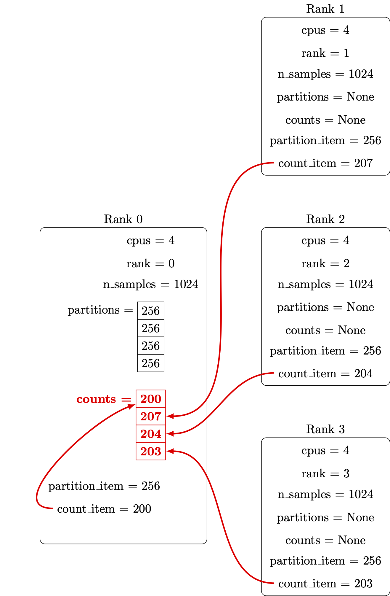
Print out the report:

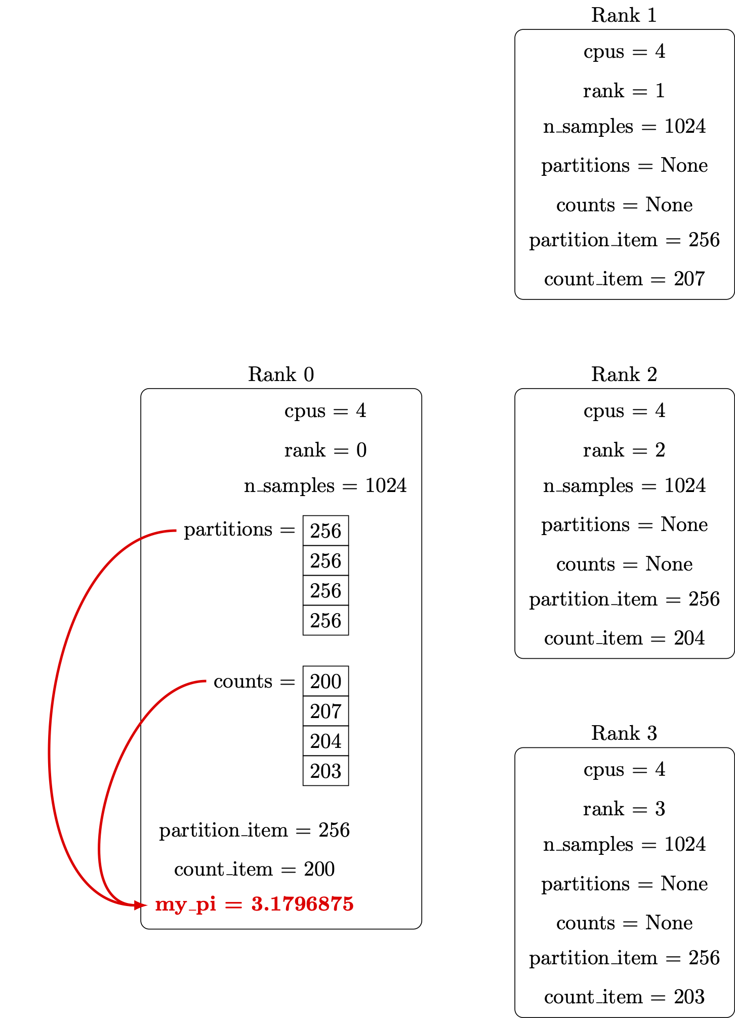
Finally, we’ll ensure the my_pi through print lines only run on rank 0. Otherwise, every parallel processor will print its local value, and the report will become hopelessly garbled:

if rank == 0:
   my_pi = 4.0 * sum(counts) / sum(partitions)
   end_time = datetime.datetime.now()
   elapsed_time = (end_time - start_time).total_seconds()
   size_of_float = np.dtype(np.float64).itemsize
   memory_required = 3 * sum(partitions) * size_of_float / (1024**3)
   print("Pi: {}, memory: {} GiB, time: {} s".format(my_pi, memory_required,
                                                            elapsed_time))

A fully commented version of the final MPI parallel python code is available here.

Our purpose here is to exercise the parallel workflow of the cluster, not to optimize the program to minimize its memory footprint. Rather than push our local machines to the breaking point (or, worse, the login node), let’s give it to a cluster node with more resources.

Create a submission file, requesting more than one task on a single node:

[yourUsername@login-1.SAGA ~]$ nano parallel-pi.sh
[yourUsername@login-1.SAGA ~]$ cat parallel-pi.sh

#SBATCH --job-name=serial-pi
#SBATCH --account=<YourAccount>
#SBATCH --time=1:00:00
#SBATCH --qos=devel
#SBATCH --nodes=1
#SBATCH --ntasks=4
#SBATCH --mem=3G

# Load the computing environment we need
module purge
module load SciPy-bundle/2021.05-foss-2021a

# Execute the task

srun python3 pi-mpi.py 100000000

Then submit your job. We will use the batch file to set the options, rather than the command line.

[yourUsername@login-1.SAGA ~]$ sbatch parallel-pi.sh

As before, use the status commands to check when your job runs. Use ls to locate the output file, and examine it. Is it what you expected?

• How good is the value for π?
• How much memory did it need?
• How much faster was this run than the serial run with 100000000 points?

Modify the job script to increase both the number of samples and the amount of memory requested (perhaps by a factor of 2, then by a factor of 10), and resubmit the job each time. You can also increase the number of CPUs.

• How good is the value for π?
• How much memory did it need?
• How long did the job take to run?

How Much Does MPI Improve Performance?

In theory, by dividing up the π calculations among n MPI processes, we should see run times reduce by a factor of n. In practice, some time is required to start the additional MPI processes, for the MPI processes to communicate and coordinate, and some types of calculations may only be able to run effectively on a single CPU.

Additionally, if the MPI processes operate on different physical CPUs in the computer, or across multiple compute nodes, additional time is required for communication compared to all processes operating on a single CPU.

Amdahl’s Law is one way of predicting improvements in execution time for a fixed parallel workload. If a workload needs 20 hours to complete on a single core, and one hour of that time is spent on tasks that cannot be parallelized, only the remaining 19 hours could be parallelized. Even if an infinite number of cores were used for the parallel parts of the workload, the total run time cannot be less than one hour.

In practice, it’s common to evaluate the parallelism of an MPI program by

• running the program across a range of CPU counts,
• recording the execution time on each run,
• comparing each execution time to the time when using a single CPU.

The speedup factor S is calculated as the single-CPU execution time divided by the multi-CPU execution time. For a laptop with 8 cores, the graph of speedup factor versus number of cores used shows relatively consistent improvement when using 2, 4, or 8 cores, but using additional cores shows a diminishing return.

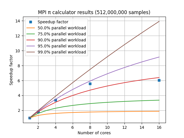
For a set of HPC nodes containing 28 cores each, the graph of speedup factor versus number of cores shows consistent improvements up through three nodes and 84 cores, but worse performance when adding a fourth node with an additional 28 cores. This is due to the amount of communication and coordination required among the MPI processes requiring more time than is gained by reducing the amount of work each MPI process has to complete. This communication overhead is not included in Amdahl’s Law.

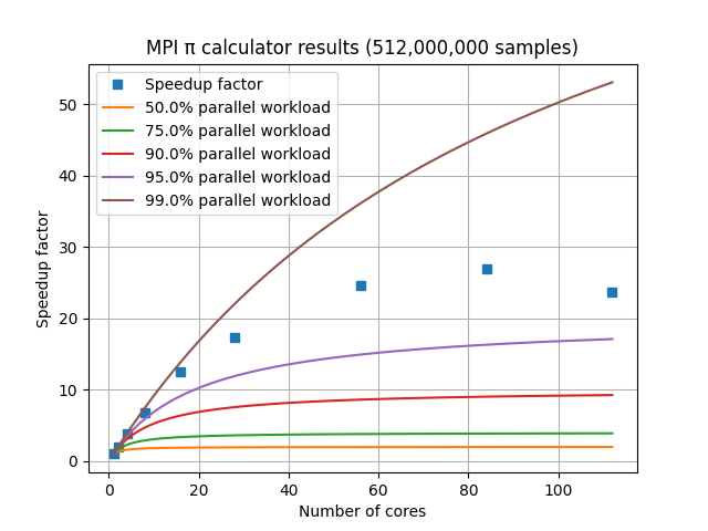
In practice, MPI speedup factors are influenced by:

• CPU design,
• the communication network between compute nodes,
• the MPI library implementations, and
• the details of the MPI program itself.

In an HPC environment, we try to reduce the execution time for all types of jobs, and MPI is an extremely common way to combine dozens, hundreds, or thousands of CPUs into solving a single problem.

Key Points

• Parallelism is an important feature of HPC clusters.

• MPI parallelism is a common case.

• The queuing system facilitates executing parallel tasks.

Using resources effectively

Overview

Teaching: 10 min
Exercises: 30 min

Questions

• How do we monitor our jobs?

• How can I get my jobs scheduled more easily?

Objectives

• Understand how to look up job statistics and profile code.

• Understand job size implications.

We’ve touched on all the skills you need to interact with an HPC cluster: logging in over SSH, loading software modules, submitting parallel jobs, and finding the output. Let’s learn about estimating resource usage and why it might matter.

Estimating Required Resources Using the Scheduler

Although we covered requesting resources from the scheduler earlier with the π code, how do we know what type of resources the software will need in the first place, and its demand for each? In general, unless the software documentation or user testimonials provide some idea, we won’t know how much memory or compute time a program will need.

Read the Documentation

Most HPC facilities maintain documentation as a wiki, a website, or a document sent along when you register for an account. Take a look at these resources, and search for the software you plan to use: somebody might have written up guidance for getting the most out of it.

A convenient way of figuring out the resources required for a job to run successfully is to submit a test job, and then ask the scheduler about its impact using sacct -u $USER. You can use this knowledge to set up the next job with a closer estimate of its load on the system. A good general rule is to ask the scheduler for 20% to 30% more time and memory than you expect the job to need. This ensures that minor fluctuations in run time or memory use will not result in your job being cancelled by the scheduler. Keep in mind that if you ask for too much, your job may not run even though enough resources are available, because the scheduler will be waiting for other people’s jobs to finish and free up the resources needed to match what you asked for.

Stats

Since we already submitted pi.py to run on the cluster, we can query the scheduler to see how long our job took and what resources were used. We will use sacct -u $USER to get statistics about parallel-pi.sh.

[yourUsername@login-1.SAGA ~]$ sacct -u $USER

       JobID    JobName  Partition    Account  AllocCPUS      State ExitCode
------------ ---------- ---------- ---------- ---------- ---------- --------
991167         Sxxxx     normal    nn9299k        128    COMPLETED      0:0

This shows all the jobs we ran recently (note that there are multiple entries per job). To get info about a specific job, we change command slightly.

[yourUsername@login-1.SAGA ~]$ sacct -u $USER -l -j 1965

It will show a lot of info, in fact, every single piece of info collected on your job by the scheduler. It may be useful to redirect this information to less to make it easier to view (use the left and right arrow keys to scroll through fields).

[yourUsername@login-1.SAGA ~]$ sacct -u $USER -l -j 1965 | less

Some interesting fields include the following:

• Hostname: Where did your job run?
• MaxRSS: What was the maximum amount of memory used?
• Elapsed: How long did the job take?
• State: What is the job currently doing/what happened to it?
• MaxDiskRead: Amount of data read from disk.
• MaxDiskWrite: Amount of data written to disk.

Measuring the System Load From Currently Running Tasks

Typically, clusters allow users to connect directly to compute nodes from the head node. This is useful to check on a running job and see how it’s doing, but is not a recommended practice in general, because it bypasses the resource manager. To reduce the risk of interfering with other users, some clusters will only allow you to connect to nodes on which you have running jobs. Let’s practice by taking a look at what’s running on the login node right now.

Monitor System Processes With top

The most reliable way to check current system stats is with top. Some sample output might look like the following (type q to exit top):

[yourUsername@login-1.SAGA ~]$ top

top - 21:00:19 up  3:07,  1 user,  load average: 1.06, 1.05, 0.96
Tasks: 311 total,   1 running, 222 sleeping,   0 stopped,   0 zombie
%Cpu(s):  7.2 us,  3.2 sy,  0.0 ni, 89.0 id,  0.0 wa,  0.2 hi,  0.2 si,  0.0 st
KiB Mem : 16303428 total,  8454704 free,  3194668 used,  4654056 buff/cache
KiB Swap:  8220668 total,  8220668 free,        0 used. 11628168 avail Mem

  PID USER      PR  NI    VIRT    RES    SHR S  %CPU %MEM     TIME+ COMMAND
 1693 jeff      20   0 4270580 346944 171372 S  29.8  2.1   9:31.89 gnome-shell
 3140 jeff      20   0 3142044 928972 389716 S  27.5  5.7  13:30.29 Web Content
 3057 jeff      20   0 3115900 521368 231288 S  18.9  3.2  10:27.71 firefox
 6007 jeff      20   0  813992 112336  75592 S   4.3  0.7   0:28.25 tilix
 1742 jeff      20   0  975080 164508 130624 S   2.0  1.0   3:29.83 Xwayland
    1 root      20   0  230484  11924   7544 S   0.3  0.1   0:06.08 systemd
   68 root      20   0       0      0      0 I   0.3  0.0   0:01.25 kworker/4:1
 2913 jeff      20   0  965620  47892  37432 S   0.3  0.3   0:11.76 code
    2 root      20   0       0      0      0 S   0.0  0.0   0:00.02 kthreadd

Overview of the most important fields:

• PID: What is the numerical id of each process?
• USER: Who started the process?
• RES: What is the amount of memory currently being used by a process (in bytes)?
• %CPU: How much of a CPU is each process using? Values higher than 100 percent indicate that a process is running in parallel.
• %MEM: What percent of system memory is a process using?
• TIME+: How much CPU time has a process used so far? Processes using 2 CPUs accumulate time at twice the normal rate.
• COMMAND: What command was used to launch a process?

htop provides an overlay for top using curses, producing a better-organized and “prettier” dashboard in your terminal. Unfortunately, it is not always available. If this is the case, ask your system administrators to install it for you. Don’t be shy, they’re here to help!

[yourUsername@login-1.SAGA ~]$ htop

ps

To show all processes from your current session, type ps.

[yourUsername@login-1.SAGA ~]$ ps

  PID TTY          TIME CMD
15113 pts/5    00:00:00 bash
15218 pts/5    00:00:00 ps

Note that this will only show processes from our current session. To show all processes you own (regardless of whether they are part of your current session or not), you can use ps ux.

[yourUsername@login-1.SAGA ~]$ ps ux

    USER       PID %CPU %MEM    VSZ   RSS TTY      STAT START   TIME COMMAND
MY_USER_NAME  67780  0.0  0.0 149140  1724 pts/81   R+   13:51   0:00 ps ux
MY_USER_NAME  73083  0.0  0.0 142392  2136 ?        S    12:50   0:00 sshd: MY_USER_NAME@pts/81
MY_USER_NAME  73087  0.0  0.0 114636  3312 pts/81   Ss   12:50   0:00 -bash

This is useful for identifying which processes are doing what.

Key Points

• The smaller your job, the faster it will schedule.

Using shared resources responsibly

Overview

Teaching: 15 min
Exercises: 5 min

Questions

• How can I be a responsible user?

• How can I protect my data?

• How can I best get large amounts of data off an HPC system?

Objectives

• Learn how to be a considerate shared system citizen.

• Understand how to protect your critical data.

• Appreciate the challenges with transferring large amounts of data off HPC systems.

• Understand how to convert many files to a single archive file using tar.

One of the major differences between using remote HPC resources and your own system (e.g. your laptop) is that remote resources are shared. How many users the resource is shared between at any one time varies from system to system but it is unlikely you will ever be the only user logged into or using such a system.

The widespread usage of scheduling systems where users submit jobs on HPC resources is a natural outcome of the shared nature of these resources. There are other things you, as an upstanding member of the community, need to consider.

Be Kind to the Login Nodes

The login node is often busy managing all of the logged in users, creating and editing files and compiling software. If the machine runs out of memory or processing capacity, it will become very slow and unusable for everyone. While the machine is meant to be used, be sure to do so responsibly — in ways that will not adversely impact other users’ experience.

Login nodes are always the right place to launch jobs. Cluster policies vary, but they may also be used for proving out workflows, and in some cases, may host advanced cluster-specific debugging or development tools. The cluster may have modules that need to be loaded, possibly in a certain order, and paths or library versions that differ from your laptop, and doing an interactive test run on the head node is a quick and reliable way to discover and fix these issues.

Login Nodes Are a Shared Resource

Remember, the login node is shared with all other users and your actions could cause issues for other people. Think carefully about the potential implications of issuing commands that may use large amounts of resource.

Unsure? Ask your friendly systems administrator (“sysadmin”) if the thing you’re contemplating is suitable for the login node, or if there’s another mechanism to get it done safely.

You can always use the commands top and ps ux to list the processes that are running on the login node along with the amount of CPU and memory they are using. If this check reveals that the login node is somewhat idle, you can safely use it for your non-routine processing task. If something goes wrong — the process takes too long, or doesn’t respond — you can use the kill command along with the PID to terminate the process.

Login Node Etiquette

Which of these commands would be a routine task to run on the login node?

1. python physics_sim.py
2. make
3. create_directories.sh
4. molecular_dynamics_2
5. tar -xzf R-3.3.0.tar.gz

Solution

Building software, creating directories, and unpacking software are common and acceptable > tasks for the login node: options #2 (make), #3 (mkdir), and #5 (tar) are probably OK. Note that script names do not always reflect their contents: before launching #3, please less create_directories.sh and make sure it’s not a Trojan horse.

Running resource-intensive applications is frowned upon. Unless you are sure it will not affect other users, do not run jobs like #1 (python) or #4 (custom MD code). If you’re unsure, ask your friendly sysadmin for advice.

If you experience performance issues with a login node you should report it to the system staff (usually via the helpdesk) for them to investigate.

Test Before Scaling

Remember that you are generally charged for usage on shared systems. A simple mistake in a job script can end up costing a large amount of resource budget. Imagine a job script with a mistake that makes it sit doing nothing for 24 hours on 1000 cores or one where you have requested 2000 cores by mistake and only use 100 of them! This problem can be compounded when people write scripts that automate job submission (for example, when running the same calculation or analysis over lots of different parameters or files). When this happens it hurts both you (as you waste lots of charged resource) and other users (who are blocked from accessing the idle compute nodes).

On very busy resources you may wait many days in a queue for your job to fail within 10 seconds of starting due to a trivial typo in the job script. This is extremely frustrating! Most systems provide dedicated resources for testing that have short wait times to help you avoid this issue.

Test Job Submission Scripts That Use Large Amounts of Resources

Before submitting a large run of jobs, submit one as a test first to make sure everything works as expected.

Before submitting a very large or very long job submit a short truncated test to ensure that the job starts as expected.

Have a Backup Plan

Although many HPC systems keep backups, it does not always cover all the file systems available and may only be for disaster recovery purposes (i.e. for restoring the whole file system if lost rather than an individual file or directory you have deleted by mistake). Protecting critical data from corruption or deletion is primarily your responsibility: keep your own backup copies.

Version control systems (such as Git) often have free, cloud-based offerings (e.g., GitHub and GitLab) that are generally used for storing source code. Even if you are not writing your own programs, these can be very useful for storing job scripts, analysis scripts and small input files.

For larger amounts of data, you should make sure you have a robust system in place for taking copies of critical data off the HPC system wherever possible to backed-up storage. Tools such as rsync can be very useful for this.

Your access to the shared HPC system will generally be time-limited so you should ensure you have a plan for transferring your data off the system before your access finishes. The time required to transfer large amounts of data should not be underestimated and you should ensure you have planned for this early enough (ideally, before you even start using the system for your research).

In all these cases, the helpdesk of the system you are using should be able to provide useful guidance on your options for data transfer for the volumes of data you will be using.

Your Data Is Your Responsibility

Make sure you understand what the backup policy is on the file systems on the system you are using and what implications this has for your work if you lose your data on the system. Plan your backups of critical data and how you will transfer data off the system throughout the project.

Transferring Data

As mentioned above, many users run into the challenge of transferring large amounts of data off HPC systems at some point (this is more often in transferring data off than onto systems but the advice below applies in either case). Data transfer speed may be limited by many different factors so the best data transfer mechanism to use depends on the type of data being transferred and where the data is going.

The components between your data’s source and destination have varying levels of performance, and in particular, may have different capabilities with respect to bandwidth and latency.

Bandwidth is generally the raw amount of data per unit time a device is capable of transmitting or receiving. It’s a common and generally well-understood metric.

Latency is a bit more subtle. For data transfers, it may be thought of as the amount of time it takes to get data out of storage and into a transmittable form. Latency issues are the reason it’s advisable to execute data transfers by moving a small number of large files, rather than the converse.

Some of the key components and their associated issues are:

• Disk speed: File systems on HPC systems are often highly parallel, consisting of a very large number of high performance disk drives. This allows them to support a very high data bandwidth. Unless the remote system has a similar parallel file system you may find your transfer speed limited by disk performance at that end.
• Meta-data performance: Meta-data operations such as opening and closing files or listing the owner or size of a file are much less parallel than read/write operations. If your data consists of a very large number of small files you may find your transfer speed is limited by meta-data operations. Meta-data operations performed by other users of the system can also interact strongly with those you perform so reducing the number of such operations you use (by combining multiple files into a single file) may reduce variability in your transfer rates and increase transfer speeds.
• Network speed: Data transfer performance can be limited by network speed. More importantly it is limited by the slowest section of the network between source and destination. If you are transferring to your laptop/workstation, this is likely to be its connection (either via LAN or WiFi).
• Firewall speed: Most modern networks are protected by some form of firewall that filters out malicious traffic. This filtering has some overhead and can result in a reduction in data transfer performance. The needs of a general purpose network that hosts email/web-servers and desktop machines are quite different from a research network that needs to support high volume data transfers. If you are trying to transfer data to or from a host on a general purpose network you may find the firewall for that network will limit the transfer rate you can achieve.

As mentioned above, if you have related data that consists of a large number of small files it is strongly recommended to pack the files into a larger archive file for long term storage and transfer. A single large file makes more efficient use of the file system and is easier to move, copy and transfer because significantly fewer metadata operations are required. Archive files can be created using tools like tar and zip. We have already met tar when we talked about data transfer earlier.

Consider the Best Way to Transfer Data

If you are transferring large amounts of data you will need to think about what may affect your transfer performance. It is always useful to run some tests that you can use to extrapolate how long it will take to transfer your data.

Say you have a “data” folder containing 10,000 or so files, a healthy mix of small and large ASCII and binary data. Which of the following would be the best way to transfer them to saga?

1. [user@laptop ~]$ scp -r data MY_USER_NAME@saga.sigma2.no:~/
   

2. [user@laptop ~]$ rsync -ra data MY_USER_NAME@saga.sigma2.no:~/
   

3. [user@laptop ~]$ rsync -raz data MY_USER_NAME@saga.sigma2.no:~/
   

4. [user@laptop ~]$ tar -cvf data.tar data
   [user@laptop ~]$ rsync -raz data.tar MY_USER_NAME@saga.sigma2.no:~/
   

5. [user@laptop ~]$ tar -cvzf data.tar.gz data
   [user@laptop ~]$ rsync -ra data.tar.gz MY_USER_NAME@saga.sigma2.no:~/
   

Solution

1. scp will recursively copy the directory. This works, but without compression.
2. rsync -ra works like scp -r, but preserves file information like creation times. This is marginally better.
3. rsync -raz adds compression, which will save some bandwidth. If you have a strong CPU at both ends of the line, and you’re on a slow network, this is a good choice.
4. This command first uses tar to merge everything into a single file, then rsync -z to transfer it with compression. With this large number of files, metadata overhead can hamper your transfer, so this is a good idea.
5. This command uses tar -z to compress the archive, then rsync to transfer it. This may perform similarly to #4, but in most cases (for large datasets), it’s the best combination of high throughput and low latency (making the most of your time and network connection).

Key Points

• Be careful how you use the login node.

• Your data on the system is your responsibility.

• Plan and test large data transfers.

• It is often best to convert many files to a single archive file before transferring.

• Again, don’t run stuff on the login node.