Running a parallel job

Overview

Teaching: 30 min
Exercises: 30 min

Questions

How do we execute a task in parallel?

Objectives

Understand how to run a parallel job on a cluster.

We now have the tools we need to run a multi-processor job. This is a very important aspect of HPC systems, as parallelism is one of the primary tools we have to improve the performance of computational tasks.

Our example implements a stochastic algorithm for estimating the value of π, the ratio of the circumference to the diameter of a circle. The program generates a large number of random points on a 1×1 square centered on (½,½), and checks how many of these points fall inside the unit circle. On average, π/4 of the randomly-selected points should fall in the circle, so π can be estimated from 4f, where f is the observed fraction of points that fall in the circle. Because each sample is independent, this algorithm is easily implemented in parallel.

/hpc-intro/Algorithm%20for%20computing%20pi%20through%20random%20sampling

A Serial Solution to the Problem

We start from a Python script using concepts taught in Software Carpentry’s Programming with Python workshops. We want to allow the user to specify how many random points should be used to calculate π through a command-line parameter. This script will only use a single CPU for its entire run, so it’s classified as a serial process.

Let’s write a Python program, pi.py, to estimate π for us. Start by importing the numpy module for calculating the results, and the sys module to process command-line parameters:

import numpy as np
import sys

We define a Python function inside_circle that accepts a single parameter for the number of random points used to calculate π. See Programming with Python: Creating Functions for a review of Python functions. It randomly samples points with both x and y on the half-open interval [0, 1). It then computes their distances from the origin (i.e., radii), and returns how many of those distances were less than or equal to 1.0. All of this is done using vectors of double-precision (64-bit) floating-point values.

def inside_circle(total_count):
    x = np.random.uniform(size=total_count)
    y = np.random.uniform(size=total_count)
    radii = np.sqrt(x*x + y*y)
    count = len(radii[np.where(radii<=1.0)])
    return count

Next, we create a main function to call the inside_circle function and calculate π from its returned result. See Programming with Python: Command-Line Programs for a review of main functions and parsing command-line parameters.

def main():
    n_samples = int(sys.argv[1])
    counts = inside_circle(n_samples)
    my_pi = 4.0 * counts / n_samples
    print(my_pi)

if __name__ == '__main__':
    main()

If we run the Python script locally with a command-line parameter, as in python pi-serial.py 1024, we should see the script print its estimate of π:

[user@laptop ~]$ python pi-serial.py 1024
3.10546875

Random Number Generation

In the preceding code, random numbers are conveniently generated using the built-in capabilities of NumPy. In general, random-number generation is difficult to do well, it’s easy to accidentally introduce correlations into the generated sequence.

Discuss why generating high quality random numbers might be difficult.

Is the quality of random numbers generated sufficient for estimating π in this implementation?

Solution

Computers are deterministic and produce pseudo random numbers using an algorithm. The choice of algorithm and its parameters determines how random the generated numbers are. Pseudo random number generation algorithms usually produce a sequence numbers taking the previous output as an input for generating the next number. At some point the sequence of pseudo random numbers will repeat, so care is required to make sure the repetition period is long and that the generated numbers have statistical properties similar to those of true random numbers.

Yes.

Measuring Performance of the Serial Solution

The stochastic method used to estimate π should converge on the true value as the number of random points increases. But as the number of points increases, creating the variables x, y, and radii requires more time and more memory. Eventually, the memory required may exceed what’s available on our local laptop or desktop, or the time required may be too long to meet a deadline. So we’d like to take some measurements of how much memory and time the script requires, and later take the same measurements after creating a parallel version of the script to see the benefits of parallelizing the calculations required.

Estimating Memory Requirements

Since the largest variables in the script are x, y, and radii, each containing n_samples points, we’ll modify the script to report their total memory required. Each point in x, y, or radii is stored as a NumPy float64, we can use NumPy’s dtype function to calculate the size of a float64.

Replace the print(my_pi) line with the following:

size_of_float = np.dtype(np.float64).itemsize
memory_required = 3 * n_samples * size_of_float / (1024**3)
print("Pi: {}, memory: {} GiB".format(my_pi, memory_required))

The first line calculates the bytes of memory required for a single float64 value using the dtypefunction. The second line estimates the total amount of memory required to store three variables containing n_samples float64 values, converting the value into units of gibibytes. The third line prints both the estimate of π and the estimated amount of memory used by the script.

The updated Python script is:

import numpy as np
import sys

def inside_circle(total_count):
    x = np.random.uniform(size=total_count)
    y = np.random.uniform(size=total_count)
    radii = np.sqrt(x*x + y*y)
    count = len(radii[np.where(radii<=1.0)])
    return count

def main():
    n_samples = int(sys.argv[1])
    counts = inside_circle(n_samples)
    my_pi = 4.0 * counts / n_samples
    size_of_float = np.dtype(np.float64).itemsize
    memory_required = 3 * n_samples * size_of_float / (1024**3)
    print("Pi: {}, memory: {} GiB".format(my_pi, memory_required))

if __name__ == '__main__':
    main()

Run the script again with a few different values for the number of samples, and see how the memory required changes:

[user@laptop ~]$ python pi-serial.py 1000
Pi: 3.144, memory: 2.2351741790771484e-05 GiB
[user@laptop ~]$ python pi-serial.py 2000
Pi: 3.18, memory: 4.470348358154297e-05 GiB
[user@laptop ~]$ python pi-serial.py 1000000
Pi: 3.140944, memory: 0.022351741790771484 GiB
[user@laptop ~]$ python pi-serial.py 100000000
Pi: 3.14182724, memory: 2.2351741790771484 GiB

Here we can see that the estimated amount of memory required scales linearly with the number of samples used. In practice, there is some memory required for other parts of the script, but the x, y, and radii variables are by far the largest influence on the total amount of memory required.

Estimating Calculation Time

Most of the calculations required to estimate π are in the inside_circle function:

Generating n_samples random values for x and y.
Calculating n_samples values of radii from x and y.
Counting how many values in radii are under 1.0.

There’s also one multiplication operation and one division operation required to convert the counts value to the final estimate of π in the main function.

A simple way to measure the calculation time is to use Python’s datetime module to store the computer’s current date and time before and after the calculations, and calculate the difference between those times.

To add the time measurement to the script, add the following line below the import sys line:

import datetime

Then, add the following line immediately above the line calculating counts:

start_time = datetime.datetime.now()

Add the following two lines immediately below the line calculating counts:

end_time = datetime.datetime.now()
elapsed_time = (end_time - start_time).total_seconds()

And finally, modify the print statement with the following:

print("Pi: {}, memory: {} GiB, time: {} s".format(my_pi, memory_required,
                                                  elapsed_time))

The final Python script for the serial solution is:

import numpy as np
import sys
import datetime

def inside_circle(total_count):
    x = np.random.uniform(size=total_count)
    y = np.random.uniform(size=total_count)
    radii = np.sqrt(x*x + y*y)
    count = len(radii[np.where(radii<=1.0)])
    return count

def main():
    n_samples = int(sys.argv[1])
    start_time = datetime.datetime.now()
    counts = inside_circle(n_samples)
    my_pi = 4.0 * counts / n_samples
    end_time = datetime.datetime.now()
    elapsed_time = (end_time - start_time).total_seconds()
    size_of_float = np.dtype(np.float64).itemsize
    memory_required = 3 * n_samples * size_of_float / (1024**3)
    print("Pi: {}, memory: {} GiB, time: {} s".format(my_pi, memory_required,
                                                      elapsed_time))

if __name__ == '__main__':
    main()

Run the script again with a few different values for the number of samples, and see how the solution time changes:

[user@laptop ~]$ python pi-serial.py 1000000
Pi: 3.139612, memory: 0.022351741790771484 GiB, time: 0.034872 s
[user@laptop ~]$ python pi-serial.py 10000000
Pi: 3.1425492, memory: 0.22351741790771484 GiB, time: 0.351212 s
[user@laptop ~]$ python pi-serial.py 100000000
Pi: 3.14146608, memory: 2.2351741790771484 GiB, time: 3.735195 s

Here we can see that the amount of time required scales approximately linearly with the number of samples used. There could be some variation in additional runs of the script with the same number of samples, since the elapsed time is affected by other programs running on the computer at the same time. But if the script is the most computationally-intensive process running at the time, its calculations are the largest influence on the elapsed time.

Now that we’ve developed our initial script to estimate π, we can see that as we increase the number of samples:

The estimate of π tends to become more accurate.
The amount of memory required scales approximately linearly.
The amount of time to calculate scales approximately linearly.

In general, achieving a better estimate of π requires a greater number of points. Take a closer look at inside_circle: should we expect to get high accuracy on a single machine?

Probably not. The function allocates three arrays of size N equal to the number of points belonging to this process. Using 64-bit floating point numbers, the memory footprint of these arrays can get quite large. Each 100,000,000 points sampled consumes 2.24 GiB of memory. Sampling 400,000,000 points consumes 8.94 GiB of memory, and if your machine has less RAM than that, it will grind to a halt. If you have 16 GiB installed, you won’t quite make it to 750,000,000 points.

Running the Serial Job on a Compute Node

Create a submission file, requesting one task on a single node and enough memory to prevent the job from running out of memory:

[yourUsername@login-1.SAGA ~]$ nano serial-pi.sh
[yourUsername@login-1.SAGA ~]$ cat serial-pi.sh

#!/usr/bin/env bash
#SBATCH --job-name=serial-pi
#SBATCH --account=<YourAccount>
#SBATCH --time=1:00:00
#SBATCH --qos=devel
#SBATCH --nodes=1
#SBATCH --ntasks=1
#SBATCH --mem=3G

# Load the computing environment we need
module purge
module load SciPy-bundle/2021.05-foss-2021a

# Execute the task
python3 pi.py 100000000

Then submit your job. We will use the batch file to set the options, rather than the command line.

[yourUsername@login-1.SAGA ~]$ sbatch serial-pi.sh

As before, use the status commands to check when your job runs. Use ls to locate the output file, and examine it. Is it what you expected?

How good is the value for π?
How much memory did it need?
How long did the job take to run?

Modify the job script to increase both the number of samples and the amount of memory requested (perhaps by a factor of 2, then by a factor of 10), and resubmit the job each time.

How good is the value for π?
How much memory did it need?
How long did the job take to run?

Even with sufficient memory for necessary variables, a script could require enormous amounts of time to calculate on a single CPU. To reduce the amount of time required, we need to modify the script to use multiple CPUs for the calculations. In the largest problem scales, we could use multiple CPUs in multiple compute nodes, distributing the memory requirements across all the nodes used to calculate the solution.

Running the Parallel Job

We will run an example that uses the Message Passing Interface (MPI) for parallelism — this is a common tool on HPC systems.

What is MPI?

The Message Passing Interface is a set of tools which allow multiple parallel jobs to communicate with each other. Typically, a single executable is run multiple times, possibly on different machines, and the MPI tools are used to inform each instance of the executable about how many instances there are, which instance it is. MPI also provides tools to allow communication and coordination between instances. An MPI instance typically has its own copy of all the local variables.

While MPI jobs can generally be run as stand-alone executables, in order for them to run in parallel they must use an MPI run-time system, which is a specific implementation of the MPI standard. To do this, they should be started via a command such as srun (or mpirun, or mpiexec, etc. depending on the MPI run-time you need to use), which will ensure that the appropriate run-time support for parallelism is included.

MPI Runtime Arguments

On their own, commands such as srun can take many arguments specifying how many machines will participate in the execution, and you might need these if you would like to run an MPI program on your laptop (for example). In the context of a queuing system, however, it is frequently the case that we do not need to specify this information as the MPI run-time will have been configured to obtain it from the queuing system, by examining the environment variables set when the job is launched.

What Changes Are Needed for an MPI Version of the π Calculator?

First, we need to import the MPI object from the Python module mpi4py by adding an from mpi4py import MPI line immediately below the import datetime line.

Second, we need to modify the “main” function to perform the overhead and accounting work required to:

subdivide the total number of points to be sampled,

partition the total workload among the various parallel processors available,

have each parallel process report the results of its workload back to the “rank 0” process, which does the final calculations and prints out the result.

The modifications to the serial script demonstrate four important concepts:

COMM_WORLD: the default MPI Communicator, providing a channel for all the processes involved in this mpiexec to exchange information with one another.

Scatter: A collective operation in which an array of data on one MPI rank is divided up, with separate portions being sent out to the partner ranks. Each partner rank receives data from the matching index of the host array.

Gather: The inverse of scatter. One rank populates a local array, with the array element at each index assigned the value provided by the corresponding partner rank — including the host’s own value.

Conditional Output: since every rank is running the same code, the partitioning, the final calculations, and the print statement are wrapped in a conditional so that only one rank performs these operations.

We add the lines:

comm = MPI.COMM_WORLD
cpus = comm.Get_size()
rank = comm.Get_rank()

immediately before the n_samples line to set up the MPI environment for each process.

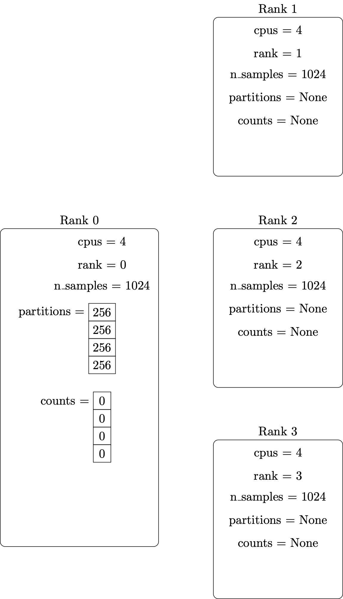
We replace the start_time and counts lines with the lines:

if rank == 0:
  start_time = datetime.datetime.now()
  partitions = [ int(n_samples / cpus) ] * cpus
  counts = [ int(0) ] * cpus
else:
  partitions = None
  counts = None

This ensures that only the rank 0 process measures times and coordinates the work to be distributed to all the ranks, while the other ranks get placeholder values for the partitions and counts variables.

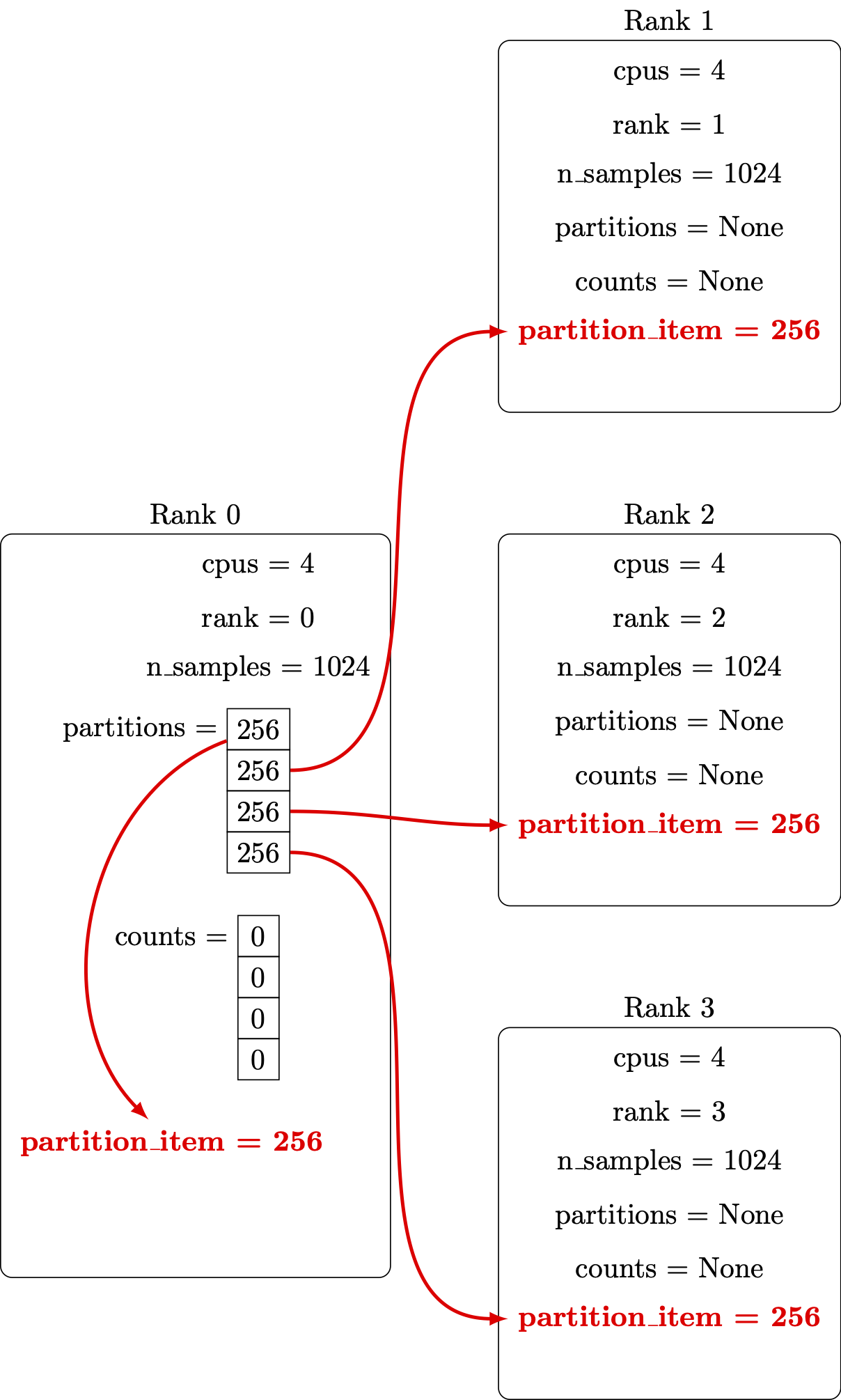
Immediately below these lines, let’s

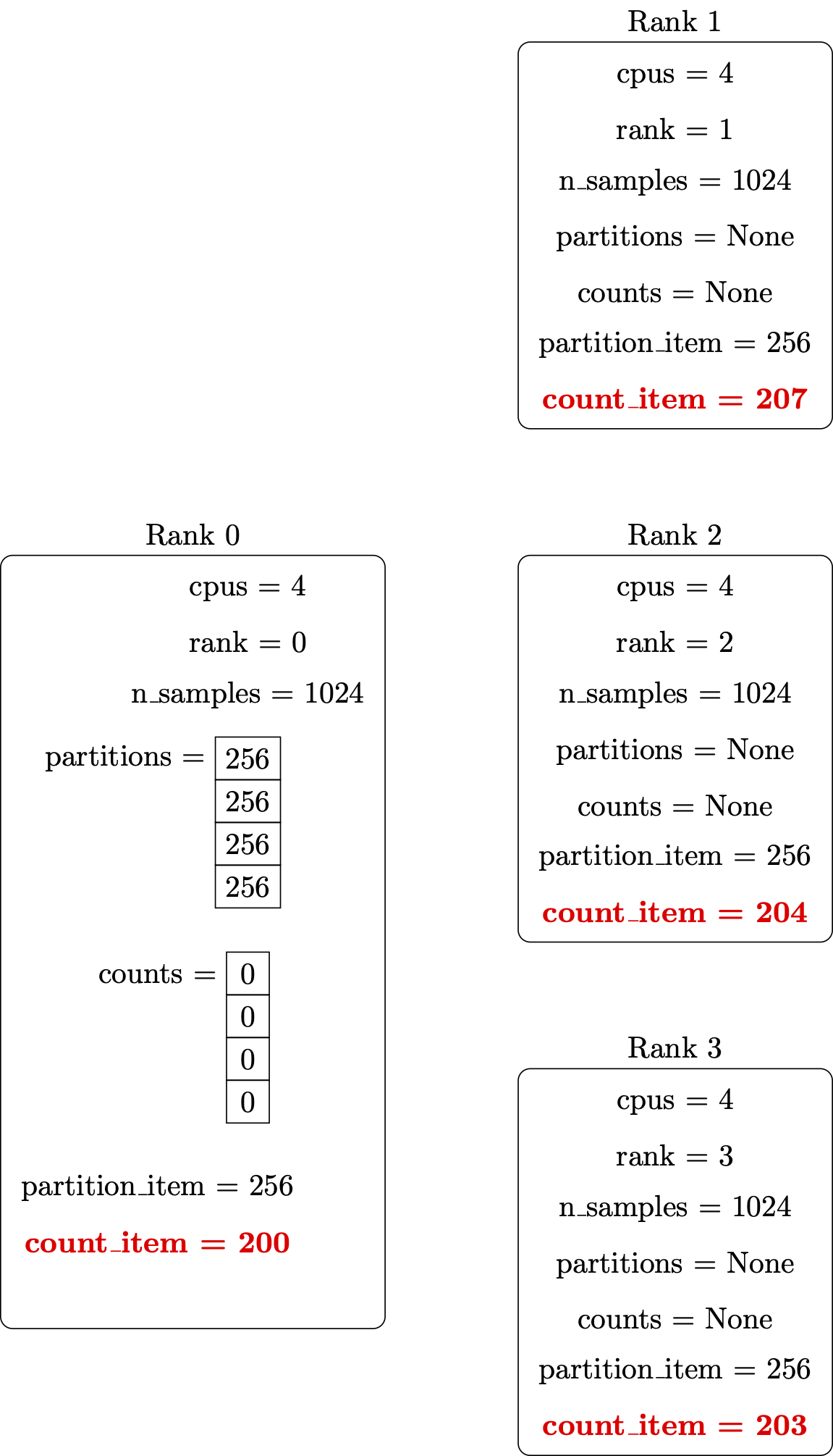
distribute the work among the ranks with MPI scatter,
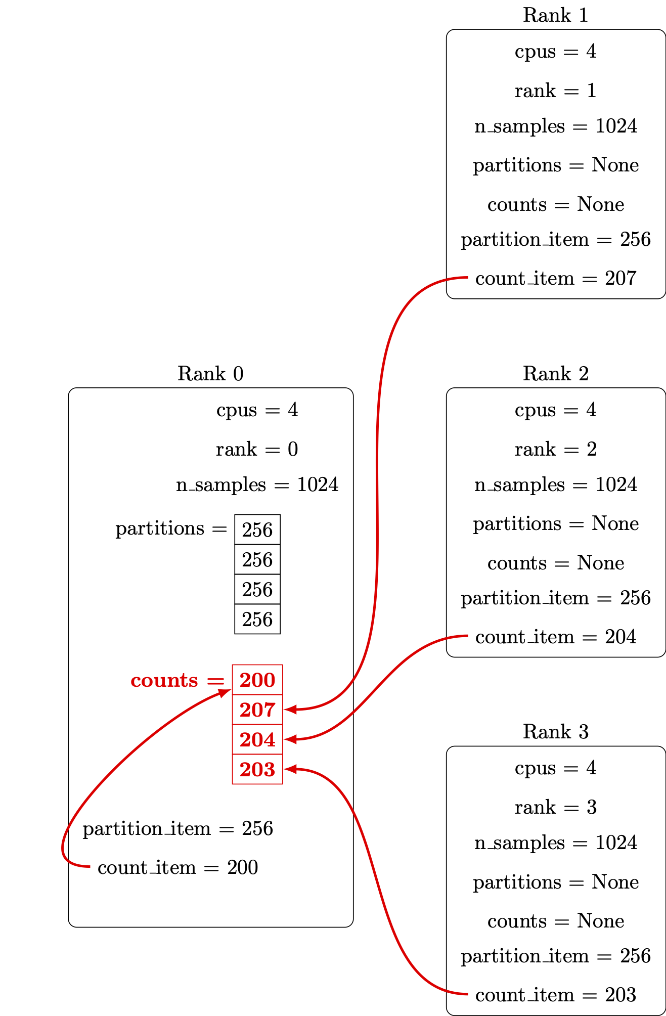
call the inside_circle function so each rank can perform its share of the work,
collect each rank’s results into a counts variable on rank 0 using MPI gather.

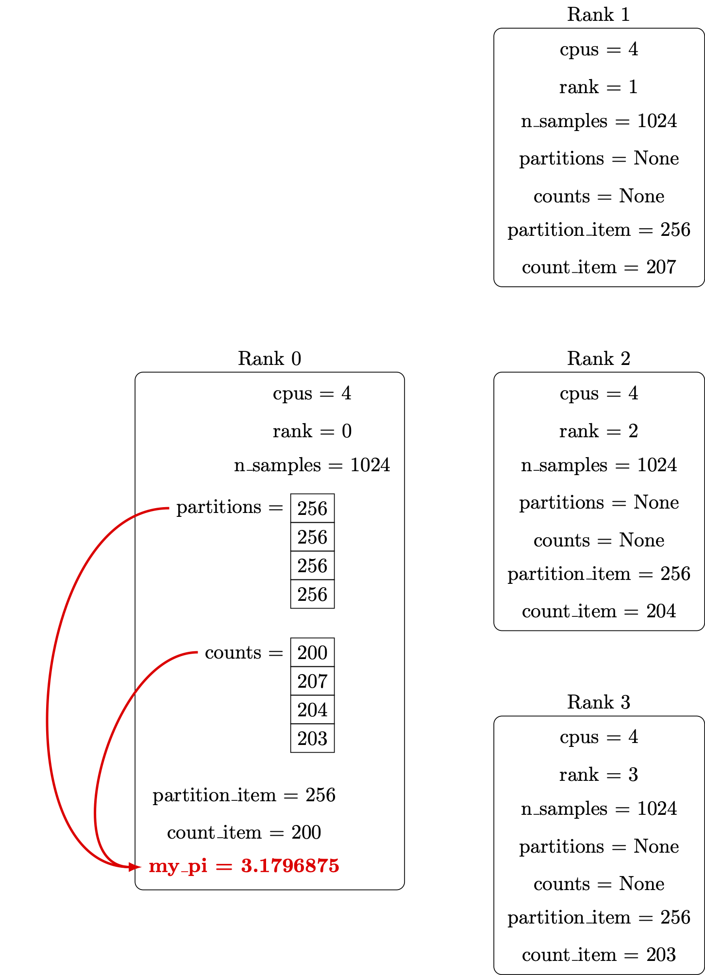
by adding the following three lines:

partition_item = comm.scatter(partitions, root=0)
count_item = inside_circle(partition_item)
counts = comm.gather(count_item, root=0)

Illustrations of these steps are shown below.

Setup the MPI environment and initialize local variables — including the vector containing the number of points to generate on each parallel processor:

Distribute the number of points from the originating vector to all the parallel processors:

Perform the computation in parallel:

Retrieve counts from all the parallel processes:

Print out the report:

Finally, we’ll ensure the my_pi through print lines only run on rank 0. Otherwise, every parallel processor will print its local value, and the report will become hopelessly garbled:

if rank == 0:
   my_pi = 4.0 * sum(counts) / sum(partitions)
   end_time = datetime.datetime.now()
   elapsed_time = (end_time - start_time).total_seconds()
   size_of_float = np.dtype(np.float64).itemsize
   memory_required = 3 * sum(partitions) * size_of_float / (1024**3)
   print("Pi: {}, memory: {} GiB, time: {} s".format(my_pi, memory_required,
                                                            elapsed_time))

A fully commented version of the final MPI parallel python code is available here.

Our purpose here is to exercise the parallel workflow of the cluster, not to optimize the program to minimize its memory footprint. Rather than push our local machines to the breaking point (or, worse, the login node), let’s give it to a cluster node with more resources.

Create a submission file, requesting more than one task on a single node:

[yourUsername@login-1.SAGA ~]$ nano parallel-pi.sh
[yourUsername@login-1.SAGA ~]$ cat parallel-pi.sh

#SBATCH --job-name=serial-pi
#SBATCH --account=<YourAccount>
#SBATCH --time=1:00:00
#SBATCH --qos=devel
#SBATCH --nodes=1
#SBATCH --ntasks=4
#SBATCH --mem=3G

# Load the computing environment we need
module purge
module load SciPy-bundle/2021.05-foss-2021a

# Execute the task

srun python3 pi-mpi.py 100000000

Then submit your job. We will use the batch file to set the options, rather than the command line.

[yourUsername@login-1.SAGA ~]$ sbatch parallel-pi.sh

As before, use the status commands to check when your job runs. Use ls to locate the output file, and examine it. Is it what you expected?

How good is the value for π?
How much memory did it need?
How much faster was this run than the serial run with 100000000 points?

Modify the job script to increase both the number of samples and the amount of memory requested (perhaps by a factor of 2, then by a factor of 10), and resubmit the job each time. You can also increase the number of CPUs.

How good is the value for π?
How much memory did it need?
How long did the job take to run?

How Much Does MPI Improve Performance?

In theory, by dividing up the π calculations among n MPI processes, we should see run times reduce by a factor of n. In practice, some time is required to start the additional MPI processes, for the MPI processes to communicate and coordinate, and some types of calculations may only be able to run effectively on a single CPU.

Additionally, if the MPI processes operate on different physical CPUs in the computer, or across multiple compute nodes, additional time is required for communication compared to all processes operating on a single CPU.

Amdahl’s Law is one way of predicting improvements in execution time for a fixed parallel workload. If a workload needs 20 hours to complete on a single core, and one hour of that time is spent on tasks that cannot be parallelized, only the remaining 19 hours could be parallelized. Even if an infinite number of cores were used for the parallel parts of the workload, the total run time cannot be less than one hour.

In practice, it’s common to evaluate the parallelism of an MPI program by

running the program across a range of CPU counts,
recording the execution time on each run,
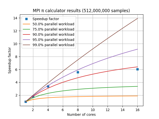
comparing each execution time to the time when using a single CPU.

The speedup factor S is calculated as the single-CPU execution time divided by the multi-CPU execution time. For a laptop with 8 cores, the graph of speedup factor versus number of cores used shows relatively consistent improvement when using 2, 4, or 8 cores, but using additional cores shows a diminishing return.

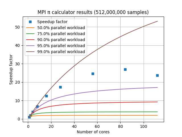
/hpc-intro/MPI%20speedup%20factors%20on%20an%208-core%20laptop

For a set of HPC nodes containing 28 cores each, the graph of speedup factor versus number of cores shows consistent improvements up through three nodes and 84 cores, but worse performance when adding a fourth node with an additional 28 cores. This is due to the amount of communication and coordination required among the MPI processes requiring more time than is gained by reducing the amount of work each MPI process has to complete. This communication overhead is not included in Amdahl’s Law.

In practice, MPI speedup factors are influenced by:

CPU design,
the communication network between compute nodes,
the MPI library implementations, and
the details of the MPI program itself.

In an HPC environment, we try to reduce the execution time for all types of jobs, and MPI is an extremely common way to combine dozens, hundreds, or thousands of CPUs into solving a single problem.

Key Points

Parallelism is an important feature of HPC clusters.

MPI parallelism is a common case.

The queuing system facilitates executing parallel tasks.

previous episode

Introduction to High-Performance Computing

next episode

Running a parallel job

Overview

A Serial Solution to the Problem

Random Number Generation

Solution

Measuring Performance of the Serial Solution

Estimating Memory Requirements

Estimating Calculation Time

Running the Serial Job on a Compute Node

Running the Parallel Job

What is MPI?

MPI Runtime Arguments

What Changes Are Needed for an MPI Version of the π Calculator?

How Much Does MPI Improve Performance?

Key Points

previous episode

next episode